Image: TYPES
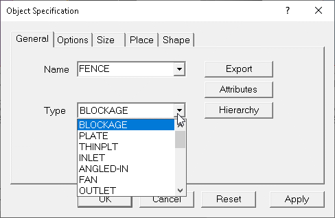
The allowable object Types are :
| Object Type | Brief Description |
| Blockage | 3D, solid or fluid. Can apply heat and momentum sources. |
| Plate | 2D, zero thickness obstacle to flow. May be porous. |
| Thin Plate | 2D, nominal thickness for heat transfer. |
| Inlet | 2D, fixed mass source. |
| Angled-in | 3D, fixed mass source on surface of underlying BLOCKAGE object. |
| Fan | 2D, fixed velocity |
| Outlet | 2D, fixed pressure. |
| Angled-out | 3D, fixed pressure on surface of underlying BLOCKAGE object. |
| Wind | 3D, whole domain, applies wind profiles at domain boundaries |
| Sun | 3D, whole domain, applies solar radiation heat load within domain. |
| Pressure Relief | single cell fixed pressure point. |
| Heat_source | 2D or 3D fluid or solid region with a heat source. |
| Foliage | 3D, represents effects of vegetation. |
| User Defined | 2D or 3D, for setting user-defined sources (PATCH/COVAL). |
| ROTOR | 3D, rotating co-ordinate zone in cylindrical-polar grid |
| Point_history | single cell monitor point. |
| Null | 2D or 3D. Used to cut the grid for mesh control. |
| Fine Grid Vol | 3D region of fine grid. |
| Transfer | 2D, transfers sources between calculations |
| Assembly | 2D or 3D container object for multi-component object |
| Clipping_plane | 3D, graphically clips the image. No effect on solution. |
| Plot_surface | 2D or 3D, provides surface for contour or vector plots in Viewer. No effect on solution. |
| Track_counter | 2D or 3D, provides surface for counting VR-Viewer streamlines or GENTRA tracks passing through. No effect on solution. |
The following object types are now deprecated, and do not appear in the list of object types. However, if a Q1 file containing any of these object types is opened, any deprecated object types will still be recognised, and they will be added to the bottom of the list.
| Object Type | Brief Description |
| Wind_Profile | 2D, fixed mass source following atmospheric boundary layer. |
| Celltype | 2D or 3D, for setting user-defined sources (cannot affect grid). |
| PCB | 3D, solid or fluid with non-isotropic thermal conductivity |
| Drag_lift | 3D, region over which momentum imbalance (force) will be calculated. |
The object type may be selected in a VR Editor session from the 'General' tab of the Object Specification dialog.
Image: TYPES
Many of the object types have a set default colour. These are listed in the relevant sections below, and also here.
An internal consistency check is performed to ensure that the object dimensionality and selected object type are consistent. VR-Editor will not allow a 2D attribute for a 3D object, or vice-versa.
Each object type may have different attributes; these are set by clicking on the Attributes button.
Blockage Material, Blockage Roughness, Blockage Wall Function, Blockage Slide Velocity, Blockage Energy Sources, Blockage Momentum Sources, Blockage Scalar Sources, Blockage Initial Values, Blockage Emissivity, InForm Commands, Solar Absorption Factor
A blockage is a volume object, which may prevent flow within itself. The default blockage material, 198 Solid with smooth-wall friction, also prevents any heat transfer within the blockage. In effect, any region occupied by such a blockage does not exist as far as the calculations are concerned.
The default geometry for a blockage is public\default\box.dat, and the default colour is grey (colour 33). This produces a grey cuboid.
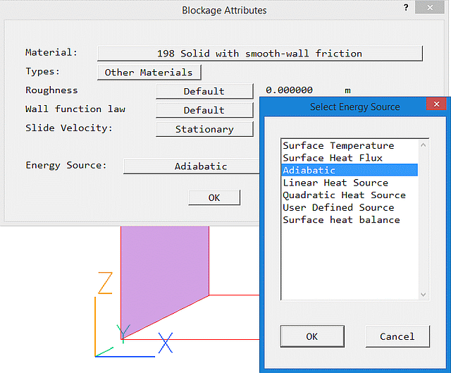
Clicking on the Attributes button for a blockage brings up the following dialog box:
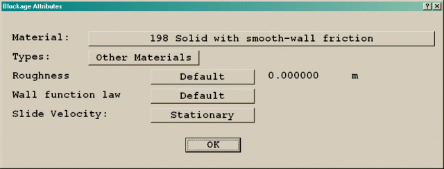
Image: ATTRIBUTES DIALOG BOX
The material a blockage is made of is set by clicking on 'Other Materials', which brings up the material type dialog box.
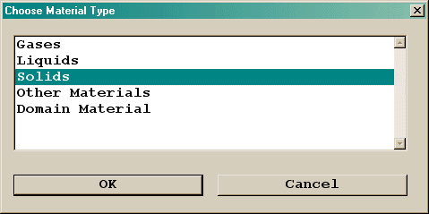
Image: OTHER MATERIAL DIALOG BOX
Selecting any of the material classes will bring up a further list of the available materials of that class. The list is read from the central property file, usually stored as \phoenics \d_earth \props. Any materials added to this file by the user will be available for selection.
If the Material of the blockage is changed to that of a 'real' solid, then the object will participate in the heat transfer calculations, should they be active, but will remain blocked to flow. If the object is made from a gas or liquid, then it will participate completely.
It is also possible to select 'Domain fluid' as the material for a blockage. This will automatically pick up whatever material has been specified in the properties panel of the main menu. A typical use of this is to 'drill' a hole through another solid. The 'drilling' object must come after the object it is making a hole in. The object order can be changed from the Object Management Dialog by right-clicking in the 'Reference' column.
Once the solid is participating in the solution, additional buttons appear which allow heat sources to be specified (if applicable). Initial values for temperature can also be set. If the blockage material is a gas or fluid, then momentum and scalar sources can be specified. Initial values can be set for pressure, velocity and solved-for scalars. Porosity values in each co-ordinate direction can be specified.
If the material is a gas or liquid, the default opaqueness is changed from 100 to 50 to make the object transparent. If a heat source has been activated, the default colour is changed to red (colour 15).
By default, solid blockages pick up the global surface roughness set in the Main Menu - Sources panel. An individual roughness height for the current object can be set.
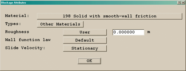
Image: OBJECT ROUGHNESS SETTING
By default, solid blockages pick up the auto wall-function coefficient set in the Main Menu - Sources panel. An individual wall-function coefficient can be set. The options are:
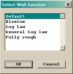
Image: OBJECT WALL-FUNCTION COEFFICIENTS
For a friction-less blockage, material 199 Solid allowing fluid-slip at walls must be selected. This material also prevents heat transfer within the blockage.
If a Wind or Wind_profile object is also being used, the wall function on any plate used to represent the ground should be set to 'Fully rough', and the roughness height set to the same value as was used for the wind velocity profile.
This option only appears for solid blockages, but not for blockages made from a fluid. By default the surfaces of the blockage are stationary. It is possible to set a non-zero surface velocity. The options for Cartesian grids are:
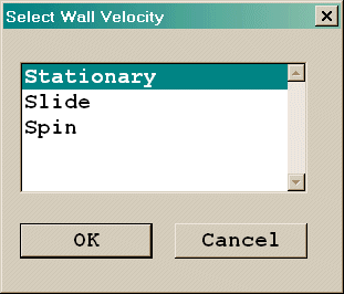
IMAGE: Slide Velocity Options
For polar grids, the options are:
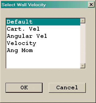
IMAGE: Polar Slide Velocity Options
The Z-direction component is always the axial velocity in m/s.
Note that these options do not cause the object to move relative to other objects and no convective effects are allowed for inside the object - they just impart moving boundary conditions on the outer surface. It is as if the object were covered with a rubber belt which was moving in the prescribed way.
Participating Solid (or Fluid)
If the energy equation is solved, then for any participating material, the following types of energy source can be selected by clicking on the Energy source entry box labeled Adiabatic:
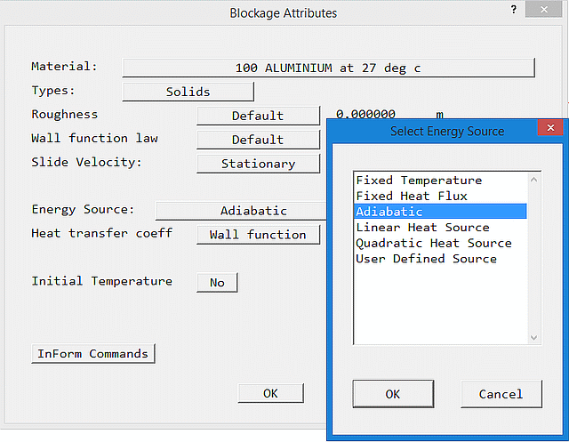
Images: ENERGY SOURCES for participating material
These are defined as:
Fixed temperature: The temperature throughout the volume of the object is fixed to the set temperature
Fixed Heat Flux: The heat flux throughout the volume of the object is fixed to the set value. The value can be specified as a total flux for the object, or as a flux per unit volume. (units W or W/m3)
Adiabatic: There is no heat source. This is the default setting for a new object.
Linear Heat Source: The heat source in any cell within the object is calculated from the expression
Q = Vol * C (V - Tp) (units of C - W/m3/K or W/m3/C, units of V - K or C)
where C and V are user-defined constants, Tp is the local cell-centre temperature, and Vol is the cell volume.
Quadratic Heat Source: The heat source is calculated from the expression
Q = Vol * C (V - Tp)2 (units of C- W/m3/K2 or W/m3/C2, units of V - K or C)
User Defined Source: The heat source is calculated from the expression
Q = Vol * C (V - Tp)
where C and/or V are calculated in the user's open-source GROUND routine and Vol is the cell volume.
The units of temperature are determined by the setting of the Reference Temperature on the Main Menu - Properties panel. If this is set to 'Kelvin', the unit of temperature is degrees Kelvin. If it is set to 'Centigrade', the temperature unit is degrees Celsius.
If IPSA is on, energy sources are set separately for each phase.
Non-Participating Faceted Solid
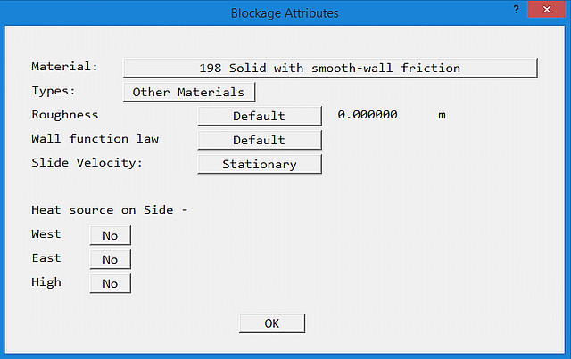
For the default non-participating (of material 198) faceted (not cuboid) blockage, it is possible to apply heat sources to the external surfaces by clicking on the Energy Source entry box labeled adiabatic:
Images: ENERGY SOURCES for non-participating faceted blockage
These are defined as:
Surface temperature: The temperature at the surface the object is set. The link between the surface temperature and the temperature in the adjacent cell is either calculated from the wall function, or can be a user-set value.
Surface Heat Flux: The heat flux over the surface of the object is fixed to the set value. The value can be specified as a total flux for the object, or as a flux per unit area. (units W or W/m2)
Adiabatic: There is no heat source. This is the default setting for a new object. Note that if the IMMERSOL radiation model is active, boundary conditions are set to ensure that the net convective + radiative heat flux is zero.
Linear Heat Source: The heat source in any cell on the surface of the object is calculated from the expression
Q = Area * C (V - Tp) (units of C - W/m2/K or W/m2/C, units of V - K or C)
where C and V are user-defined constants, Tp is the local cell-centre temperature, and Area is the surface area in the cell.
Quadratic Heat Source: The heat source is calculated from the expression
Q = Area * C (V - Tp)2 (units of C- W/m2/K2 or W/m2/C2, units of V - K or C)
User Defined Source: The heat source is calculated from the expression
Q = Area * C (V - Tp)
where C and/or V are calculated in the user's open-source GROUND routine and Area is the surface area in the cell.
Surface heat balance: The surface temperature is deduced from a heat balance between the fluid temperature in the cell adjacent to the surface, and a user-set fictitious internal temperature. The heat flux is then computed based on the surface temperature and an external heat transfer coefficient obtained from the wall function, or as a user-set constant.
Tsurf = (Ri * Tp + Rf * Tsolid)/(Ri + Rf)
where Ri is a user-set internal resistance, Rf is the fluid-side resistance (i.e. 1/heat transfer coefficient), Tp is the cell temperature and Tsolid is the user-set internal value. Note that the value entered for the 'Link coefficient' is 1/Ri.
The surface temperature can be displayed by adding STORE(TWAL). (Main Menu, Models, Solution control / Extra variables)
The heat flux is then:
Q = Area * HTCO *(Tsurf - Tp)
where Area is the surface area, HTCO is the heat transfer coefficient (from the wall function or user-set).
In transient cases, the thermal capacity of the solid is estimated from a nominal material and thickness. This is then added to the heat balance for the surface temperature:
Tsurf=(Rt*Ri*Tp+Rt*Rf*Tsolid+Ri*Rf*TsurfO)/ (Rt*Ri+Rt*Rf+Rf*Ri)
where Rt=Dt/(ρ*Cp*δ)
and Dt is the time step, ρ is a nominal density, Cp a nominal specific heat, δ a nominal thickness and TsurfO the surface temperature at the previous time step. The properties are taken from the selected nominal material:
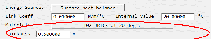
It is assumed that the user-set internal temperature Tsolid remains constant.
If the SUN object is active, the heat balance includes the solar heating.
The units of temperature are determined by the setting of the Reference Temperature on the Main Menu - Properties panel. If this is set to 'Kelvin', the unit of temperature is degrees Kelvin. If it is set to 'Centigrade', the temperature unit is degrees Celsius.
If IPSA is on, energy sources are set separately for each phase.
Non-Participating Cuboid Solid
If the blockage is a cuboid of non-participating material, heat sources can still be applied to its exposed faces.
Images: ENERGY SOURCES for non-participating cuboid blockage
By default, this is obtained from the wall-functions. Alternatively, a user-set constant value can be supplied.
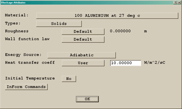
Image: BLOCKAGE HEAT TRANSFER COEFFICIENT
The values of heat transfer coefficient used can be stored into the PHI file for plotting in the Viewer. This is done from the Main Menu - Output - Derived Variables panel.
If the pressure and velocities are solved for, and the blockage is a gas or liquid, the following types of momentum source can be selected independently for each co-ordinate direction:

Image: MOMENTUM SOURCES
Fixed Velocity: The velocity throughout the volume of the object is fixed to the set value.
Fixed Momentum Flux: The momentum flux (force) throughout the volume of the object is fixed to the set value. The value is specified as a total force in Newtons for the object.
None: There is no driving force. This is the default setting for a new object.
Linear Source: The force in Newtons is calculated from the expression
F = mass-in-cell * C (V - Velp) (units of C - 1/s, units of V - m/s)
where C and V are user-defined constants, and Velp is the velocity in any cell within the object.
Quadratic Source: The force is calculated from the expression
F = mass-in-cell * C (V - Velp)2 (units of C - 1/m, units of V - m/s)
This form is suitable for representing distributed pressure losses which obey dP = K *density * velocity2, where K is an empirical constant, set as C.
User Defined Source: The force is calculated from the expression
F = mass-in-cell * C (V - Velp)
where C and/or V are calculated in the user's open-source GROUND routine
Ergun - Actual / Ergun -Superficial: The force applied is calculated from the Ergun equation for pressure-loss in a packed bed.
The force is
F = mass-in-cell* (150*ν*(1-P)2/(P3*Dp2)*(V-Velp) + 1.75*(1-P)/(Dp*P3)*Vabs*(V-Velp))
where:
For 'Actual', the porosity value is applied to the cell face areas, so the velocity is the actual device velocity. For 'Superficial', the face areas are not adjusted, and the velocity is the approach velocity. The form of the source is modified to account for this. The expression above is the 'Superficial' form.
In RESULT, the source from the linear part is reported as the source from patches with names OV, and the quadratic part as sources from patches OW.
Porous - Actual / Porous -Superficial: The force applied is calculated from an equation for pressure-loss through a porous medium allowing for viscous (linear) and inertial (quadratic) contributions.
The force is
F = Volume-of-cell*(1-P)* (ConstA*Vel + ConstB*Vel*Vabs)
where:
For 'Actual', the porosity value is applied to the cell face areas, so the velocity is the actual device velocity. For 'Superficial', the face areas are not adjusted, and the velocity is the approach velocity. The form of the source is modified to account for this. The expression above is the 'Superficial' form.
If IPSA is on, momentum sources are set separately for each phase.
If additional scalar variables (e.g. C1) are solved, and the blockage is a gas or liquid, the following types of source can be selected for any solved scalar equation:
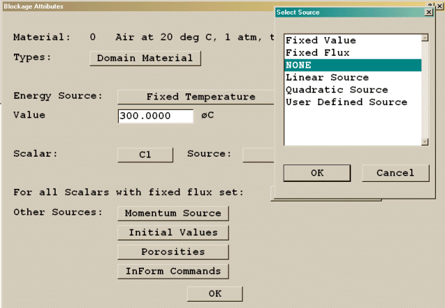
Image: SCALAR SOURCES
Further, if the name of the scalar starts with # (e.g. #C1) or the name of the scalar is EPOT, and the blockage is a participating solid, the same sources can be applied to those variables only.
Fixed value: The scalar throughout the volume of the object is fixed to the set value.
Fixed Flux: The flux throughout the volume of the object is fixed to the set value. The value can be specified as a total flux for the object, or as a flux per unit volume.
None: There is no scalar source. This is the default setting for a new object.
Linear Source: The source is calculated from the expression
S = Vol * C (V - Φp) (units of C - 1/(sVolΦ))
where C and V are user-defined constants, Φp is the scalar value in any cell within the object, and Vol is the cell volume.
Quadratic Source: The source is calculated from the expression
S = Vol * C (V - Φp)2 (units of C - 1/(sVolΦ2))
User Defined Source: The source is calculated from the expression
S = Vol * C (V - Φp)
where C and/or V are calculated in the user's open-source GROUND routine.
Initial values can be set for temperature, pressure, velocity, solved scalars and cell face and cell volume porosity factors.
If the Simple Chemically-reacting System (SCRS) is active, and an initial temperature has been set, the corresponding initial gas composition must be set as well.
If IPSA is active, initial volume fractions for Phase 1, Phase 2 and the Shadow phase (if solved) can be set.
If Algebraic Slip is active, initial particle concentrations can be set.
If either of the free-surface models, SEM or HOL, is active, the blockage can be designated as being either heavy or light fluid.
In all cases, if the Initial value button is left as No, the initial value for that quantity will be that set in the Initialisation panel of the Main Menu. If Initial value is set to Yes for pressure or temperature, the default initial value is the ambient value set on the Properties panel of the Main Menu. This can be changed to user if some other value is required.
If the IMMERSOL radiation model is active, the emissivity of a solid, or the absorption and scattering coefficients of a gas or liquid, can be set. The default emissivity is 1.0. For most substances absorption is 0.5 or greater; bricks, weathered steel and marble can be up to 0.9. The exceptions are polished metal surfaces -typically .1-.2.
This leads to a dialog from which a selection of InForm commands can be attached to this object. It is described in InForm Commands below.
When a SUN object is active an additional input box appears, in which the fraction of the incident solar radiation absorbed by this object can be set. This is a non-physical factor which can be used to diminish the amount of solar energy (specified with the Sun object) which is absorbed by the blockage surfaces. This can be used as a crude representation of diurnal effects when the Sun object is used in the context of a steady model.
Internal Plate, External Plate, Radiative Heat Loss, InForm Commands, Solar Absorption Factor, Scalar sources
A plate is a blockage, which can be treated as having zero thickness. This allows for computational efficiency, because complete cells do not have to be blocked, only cell faces. There is no heat transfer by conduction through a plate.
The default geometry for a plate is public\default\box.dat, and the default colour with no heat sources is light brown (colour 80), representing a brown rectangle.
The dialog box for an internal plate is shown below:
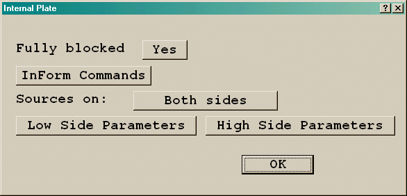
Image: INTERNAL PLATE Fully blocked
Fully blocked 'Yes' is equivalent to an area Porosity set to 0.0. If Fully blocked is set to 'No', the porosity should be set to a value greater than 0.0, and it becomes possible to set an additional pressure drop. Once the porosity is greater than 0.0, the opaqueness is reduced from100 to 50 to make the plate transparent.
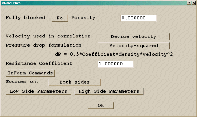
Image: INTERNAL PLATE Partial porosity
The velocity used in the pressure drop correlation can be 'Device Velocity' or 'Superficial Velocity'. 'Device Velocity' means that the porosity is applied to the flow area, so the velocity represents the velocity through the holes in the plate. 'Superficial Velocity' means that the porosity is not applied to the flow area, and the velocity represents the 'approach' velocity.
The pressure drop can be calculated from the expressions:
where Coef is the Resistance Coefficient set for the object.
The CIBSE-Guide correlations for a perforated plate and for wire mesh use formula 2) above with the following values for the resistance Coefficient:
| Free-area ratio | Coef (plate) | Coef (Mesh) |
| 0.2 | 51.0 | 17.0 |
| 0.3 | 18.0 | 6.2 |
| 0.4 | 8.3 | 3.0 |
| 0.5 | 4.0 | 1.7 |
| 0.6 | 2.0 | 1.0 |
| 0.7 | 1.0 | 0.6 |
| 0.8 | 0.4 | 0.3 |
In addition, heat transfer, scalar transfer and wall friction parameters can be specified for either side of an internal plate using the Low side parameters/High side parameters buttons.
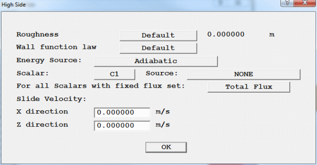
Image: HIGH SIDE PARAMETERS
The default roughness takes the equivalent sand-grain roughness height for the logarithmic wall-functions, or the roughness height for the fully-rough wall functions, from the value set in the Main menu - Sources panel (WALLA in Q1). The alternative is to set a specific value.
The default wall function coefficient is that set in the Main menu - Sources panel (WALLCO in Q1). Alternatively, it can be chosen from this list:
Image: List of wall functions
If a Wind or Wind_profile object is also being used, the wall function on any plate used to represent the ground should be set to 'Fully rough', and the roughness height set to the same value as was used for the wind velocity profile.
The energy source is specified in the same way as on a blockage, and can be different on either side of the plate. Note that the volume terms appearing in the blockage heat source expressions are all replaced by area.
Once a heat source has been set on either side, the default colour is changed to orange (colour 177).
The Slide Velocity settings allow the velocity of the surface of the plate to be set.
Plates on the outer edges of the solution domain only have the Roughness, Wall-function, Energy Source, Scalar Source and Slide Velocity settings - it is not possible to set a porosity at the domain boundary.
Image: EXTERNAL PLATE
If the IMMERSOL radiation model is active, the surface emissivity for either side of the plate can be set. For most substances emissivity is 0.5 or greater; bricks, weathered steel and marble can be up to 0.9. The exceptions are polished metal surfaces -typically .1-.2.
An external plate with IMMERSOL allows an extra energy source - Radiating Solid. This gives a heat source containing convective and radiative parts, with the form:
Q" = a + b*(Text-Tp)c + d*(Text4-Tp4)
(W/m2)
where:
a - represents a constant heat flux (W/m2)
b - represents a heat transfer coefficient in W/m2/Kc
c - represents a power
d - represents the surface emissivity * Stefan - Boltzmann constant
Text - represents the external temperature
This leads to a dialog from which a selection of InForm commands can be attached to this object. It is described in InForm Commands below.
When a SUN object is active an additional input box appears, in which the fraction of the incident solar radiation absorbed by this object can be set. The default absorption factor is 1.0 - i.e. all the heat is absorbed by the object. This is a non-physical factor which can be used to diminish the amount of solar energy (specified with the Sun object) which is absorbed by the blockage surfaces. This can be used as a crude representation of diurnal effects when the Sun object is used in the context of a steady model.
For internal plates, absorption factors are specified for each side of the plate.
If additional scalar variables (e.g. C1) are solved, the scalar source is specified in the same way as on a blockage, and can be different on either side of the plate. Note that the volume terms appearing in the blockage scalar source expressions are all replaced by area.
The scalar source can be set as a total source for the whole (side of) the plate, or as per-unit-area, but this choice applies to all scalars which have a source set.
This is similar to the PLATE type, except that heat transfer through the plate is allowed. A notional thickness and material type are specified, but these are only used for the calculation of thermal resistance.
The object must be an area. Thin plates are only allowed within the domain, but not at the edges. The default geometry for a Thin Plate is public\default\box.dat, and the default colour is light brown(colour 80) representing a brown rectangle.
The Thin Plate dialog box is shown below:
Image: FULLY BLOCKED 'YES'
If 'Fully blocked' is changed to 'No', the porosity can be set to be greater than 0.0. Once the porosity is greater than zero, the opaqueness is reduced from 100 to50 make the object transparent.
Image: FULLY BLOCKED 'NO'
The velocity and pressure drop formulations are as for the PLATE object.
If the Energy Equation is on, the initial temperature of the plate can be set.
If the IMMERSOL radiation model is on, the surface emissivity for either side of the plate can be set. For most substances emissivity is 0.5 or greater; bricks, weathered steel and marble can be up to 0.9. The exceptions are polished metal surfaces -typically .1-.2.
Solar Absorption Factor. When a SUN object is active an additional input box appears, in which the fraction of the incident solar radiation absorbed by this object can be set. The default absorption factor is 1.0 - i.e. all the heat is absorbed by the object. This is a non-physical factor which can be used to diminish the amount of solar energy (specified with the Sun object) which is absorbed by the blockage surfaces. This can be used as a crude representation of diurnal effects when the Sun object is used in the context of a steady model.
Separate absorption factors are specified for each side of the thin plate.
Single phase, Multi-phase, Radiative Heat Loss, Internal Inlets
An inlet is a region of fixed mass flow, either in or out. Inlets can only be attached to area objects.
The sign convention for velocities is that a velocity pointing in to the domain brings mass in, whilst a velocity pointing out takes mass out. For volumetric flow rate, positive flow is in to the domain, negative flow is out.
Note that if the inlet is set to extract fluid, the input boxes for external values (temperature, scalars etc.) are grayed out, as it is the local in-cell values which will be used.
The default geometry for an inlet is public\default\box.dat, the default colour is purple (colour 194), and the default opaqueness is 50, representing a transparent purple cuboid.
The basic single-phase inlet dialog box for turbulent flow is shown below:
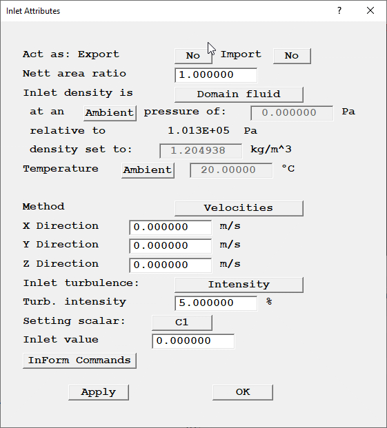
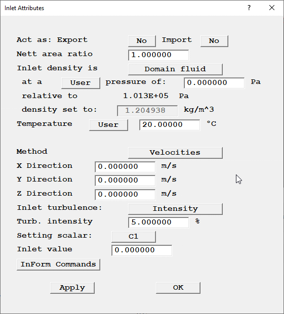
Image: SINGLE PHASE DIALOG BOX
Acts as: Export / Import allows the inlet object to behave as a Transfer Object. When Export is activated, an input box for the export file name appears. The default is the current object name. At the end of the Solver run, the named file will be created, and it will contain the mass flows and other values for all cells covered by the object.
If Import is activated, the remaining attributes are hidden, as the inflow conditions will be read from a file. The file name can either be entered into the input box, or searched for with a file browser. The default is also the current object name.
The Nett area ratio sets the ratio between the area actually available for flow, sometimes called the effective area, and the area used in the model. If the ratio is less than 1, the actual injection velocity or volumetric flow rate should be specified for the inlet condition. The mass flow will be calculated from area_ratio*velocity*density.
A density is required to calculate the mass flow rate. If the 'Inlet density is' is set to Domain fluid, the density will be taken from the formula selected for the domain fluid in the Main Menu, Properties panel. The density will be calculated from the values set at the inlet. For compressible flows, the pressure (used to calculate the density) can be the ambient pressure set in the Main Menu, Properties panel, or a user-set value.
If the fluid entering is not the domain fluid, the setting can be switched to User-set, as shown below. In this case, the required inlet density can be set directly. (This is the default for complex density relationships). This setting should also be used if InForm is used to calculate the fluid density.
The inlet Temperature (only present if the Energy Equation is active) can be switched between Ambient and User. When set to Ambient, the inlet temperature is always taken from the Ambient Temperature set on the Main Menu, Properties panel. When set to User, any required value can be entered.
The Method button switches between:
For polar grids, the options for Method are:
If the flow is turbulent, the turbulence quantities at the inlet can be set in a number of ways, controlled by the Inlet turbulence button:
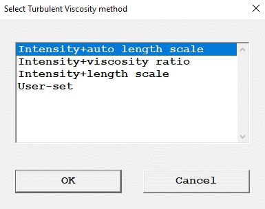
Image: INLET TURBULENCE OPTIONS
kin = (0.01*I*Vnorm)2
εin = (Cμ*Cd)3/4* kin3/2/(0.1*len)
where: I is the turbulence intensity in %;
Vnorm is the velocity normal to the inlet; and
len is the length scale, taken to be the hydraulic radius of the inlet. This is half the hydraulic diameter, which is calculated from 4*area/perimeter. The area and perimeter are always based on the bounding box of the object, so may not be accurate for a non-cuboid shape. In BFC cases len is the equivalent radius, calculated from (area/π)1/2
kin = (0.01*I*Vnorm)2
εin = (Cμ*Cd)*kin2 /(Vrat*νin)
where: I is the turbulence intensity in %;
Vnorm is the velocity normal to the inlet; and
Vrat is the ratio between the expected turbulent viscosity at the inlet and the laminar viscosity at the inlet.
kin = (0.01*I*Vnorm)2
εin = (Cμ*Cd)3/4* kin3/2/len
where: I is the turbulence intensity in %;
Vnorm is the velocity normal to the inlet; and
len is the length scale, set by the user.
Cμ, Cd are constants in the turbulence model, defaulted to 0.5478 and 0.1643 respectively. These values can be changed from the Main Menu, Models, Turbulence Models, Settings panel.
For k-ω models, the inlet values of ω are deduced from the inlet ε, or specified directly.
Note that the 'Intensity' methods are suitable for duct-type flows. Atmospheric boundary layers should be treated as described below for Wind_Profile Objects.
If the inlet values of k and ε are known, then the User-set method should be selected and the known values entered.
Inlet values for solved scalars are set by selecting the scalar with the Setting scalar button, then specifying the required inlet value.
Image: SCALAR SETTING
If the SCRS combustion model is on, a button appears which allows the inlet gas composition to be set. The enthalpy at the inlet is then deduced from the inlet temperature, gas composition and gas properties.
Note that if the reaction type is switched from mixing-controlled to kinetically-controlled, or vice-versa, the inlet gas composition values will have to be reset.
If IPSA is active, a new button appears, which allows a switch between setting values for Phase 1 or Phase 2. The Inlet density button toggles between Phase fluid and Dens*Vol frac. Phase fluid indicates that the density will be that of the current phase. Dens*Vol frac indicates that the value entered is the product of density and volume fraction.
If only one phase enters, all three velocity components or flow rates of the absent phase should be set to zero.
If Algebraic Slip is on, the Inlet density button toggles between Mixture density and User-set. Mixture density means that the inlet density will be calculated from the densities of the various particle phases and the set inlet concentrations.
If the free-surface models SEM or HOL are on, the Inlet density button toggles between Heavy fluid and Light fluid. SEM and HOL do not allow mixtures of phases at an inlet.
If the Lagrangian Particle tracker GENTRA is active, Inlets can be set to act as particle exits.
If the IMMERSOL radiation model is active, the inlet can be allowed to exchange heat by radiation with the surroundings. If the External radiative link is set to Yes, the temperature of the surroundings, Texternal, can be set. The heat flux from the inlet will then be:
Q" = σ (Text4 - Tp4) (W/m2)
where σ is the Stefan-Boltzmann constant.
If the inlet is internal to the domain, an extra button appears on the dialog box, labeled Object side. The settings for this are Low or High, and they indicate whether the inlet is to appear on the low-co-ordinate face or high-co-ordinate face of the object. The flow direction determines whether the inlet acts as a source or sink, as shown in the table below.
| Low | High | |
| Inflow | -ve velocity | +ve velocity |
| Outflow | +ve velocity | -ve velocity |
When inside the domain, INLET objects are usually located on the face of a BLOCKAGE. They represent the outflow (or inflow) from some ducting inside the blockage that is not being modeled. Positive velocity always points along the positive coordinate direction. The 'Object side HIGH/LOW' setting determines whether it represents an inflow or outflow, as in the table above.
                 --------
                 |        |
            ---->|Blockage|---->
                 |        |
                  --------
                L H      L H

                 ---------> X, Y or Z
If the setting is 'LOW', as on the left side above, the inlet acts on the smaller-coordinate side of the inlet. A positive velocity points into the blockage and thus acts as a fixed-extraction zone. If the setting is 'HIGH',as on the right side above, the inlet acts on the larger-coordinate side, and a positive velocity points out into the domain and acts as a supply. A negative velocity reverses the situation, making the left side a supply and the right an extraction.
If the setting is HIGH on the left side or LOW on the right side, the inlet acts inside the blockage and nothing happens at all.
With volume or mass flow rates, the sign convention is easier, in that positive flows are always inflow to the domain, and negative flows are always outflow from the domain.
An Angled-in is a region of fixed mass flow, either in or out. The region of influence is the part of the surface of any blockage object(s) enclosed by the angled-in object. The angled-in object itself must be a 3D volume.
The sign convention for velocities is that a velocity pointing in to the domain (i.e. away from the underlying solid) brings mass in, whilst a velocity pointing out (i.e. toward the underlying solid) takes mass out. For volumetric flow rate or mass flow rate, positive flow is in to the domain, negative flow is out.
Note that if the angled-in is set to extract fluid, the input boxes for external values (temperature, scalars etc.) are grayed out, as it is the local in-cell values which will be used.
The default geometry for an angled-inlet is public\default\box.dat, the default colour is purple (colour 194), and the default opaqueness is 50, representing a transparent purple cuboid.
The angled-in object may intersect a blockage, as shown here:
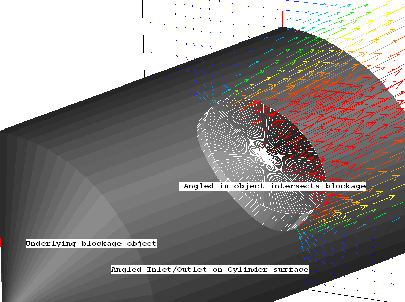
IMAGE: Angled-in intersects blockage
It may also completely surround a blockage, as shown here:
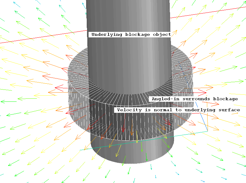
IMAGE: Angled-in surrounds blockage
Its area of influence cannot lie on the domain edge, as it must interact with a blockage.
The attributes of the Angled-in object are as those of the 'normal' inlet, with the addition of 'Normal velocity' to the methods of specifying the flow rate. This sets the velocity normal to the surface of the underlying blockage. It was used in the second example above to make the flow issue radially from the cylindrical blockage.
If the 'Intensity+ auto length-scale' method is chosen for the turbulence quantities, the inlet values are calculated from:
kin = (0.01*I*Vnorm)2
εin = (Cμ*Cd)3/4* kin3/2/(0.1*len)
where: I is the turbulence intensity in %;
Vnorm is the velocity normal to the inlet; and
len is the length scale, taken to be the equivalent radius of the inlet. This is calculated from (area/π)1/2. The hydraulic radius cannot be estimated as the perimeter is unknown in this case.
Cμ, Cd are constants in the turbulence model, defaulted to 0.5478 and 0.1643 respectively. These values can be changed from the Main Menu, Models, Turbulence Models, Settings panel.
If the inlet values of k and ε are known, then the User-set method should be selected and the known values entered.
In order to represent the flow through a piece of equipment which is not modeled in detail but is represented as a blockage, it is possible to use a pair of linked Angled-in objects.
For example, to represent an Induction Fan, one Angled-in can be used to represent the suction side of the fan. Here the extraction flow rate is specified. The nozzle of the fan is then a second Angled-in, linked to the first.
The mass flow will be taken from the first, and the temperature and other scalars will be the average values at the first. The velocity at the outflow will be deduced from the mass flow rate and the area of the outlet. If the density is set to use the Ideal Gas Law, the outlet density will be evaluated at the average outlet temperature.
The turbulence values at the outlet will be deduced from the expressions given above using the deduced velocity.
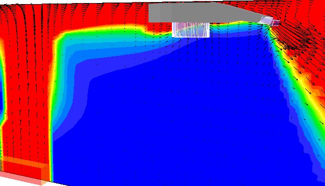
The image shows the smoke ingested by the lower intake Angled-in being ejected by the nozzle Angled-in.
In a similar way, ducting can be represented by using one Angled-in (acting as an extract) as the inlet to the duct, and a linked Angled-in as the outlet from the duct. This is demonstrated in the Tutorial ' Working with Linked Angled Inlets'.
An Angled-in can be linked to the immediately-preceding or immediately-following Angled-in. The linked Angled-ins do not need to be adjacent in the Object Management list.
Once linked, additional heat and scalar sources can be specified, representing any extra heating or cooling taking place. For the temperature equation the options are:
For scalar variables, the options are broadly similar:
The minimum and maximum allowed values of temperature and scalars at the exit from the linked pair can also be set.
Any additional energy or scalar source required to implement the change can be deduced from the energy and scalar balances printed in the 'Sources and Sinks' section of RESULT.
Limitations
Linked Angled-ins have the following limitations:
When located at the domain edges, a FAN behaves as an INLET - it acts as a source of mass. If it is located within the domain, it fixes the velocity, but does not introduce additional mass - it just circulates the fluid already present. For multi-phase flows, Fans at the domain edge must be replaced by INLET objects. Fans can only be attached to area objects.
The default geometry for a Fan is public\default\box.dat, the default colour is light grey (colour 154), and the default opaqueness is 50, representing a transparent grey cuboid. The domain-edge Fan dialog box is shown below:
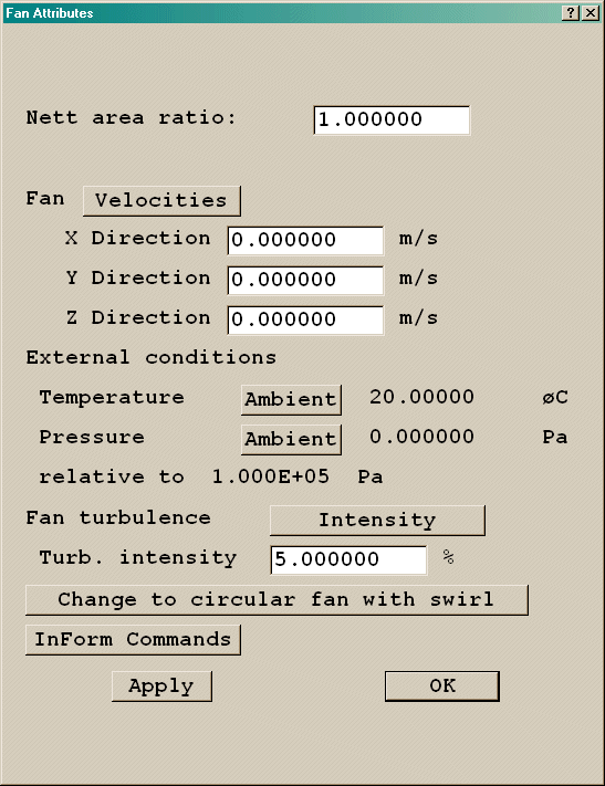
Image: DEFAULT FAN ATTRIBUTES
The Nett area ratio sets the ratio between the area actually available for flow, sometimes called the effective area, and the area used in the model. If the ratio is less than 1, the actual injection velocity or volumetric flow rate should be specified for the inlet condition. The mass flow will be calculated from area_ratio*velocity*density.
The Fan can be switched between Velocities and Vol. Flow rate, as for Inlets.
A circular fan object can be created by clicking on Change to circular fan with swirl. Circular Fans are not available in Cylindrical-polar or Body-Fitted co-ordinates.
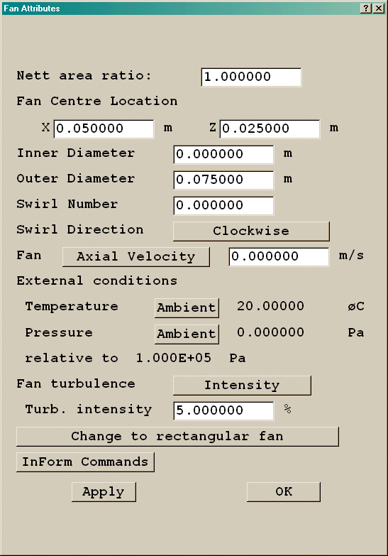
Image: CIRCULAR FAN ATTRIBUTES
The circular Fan allows for swirl, and for an inner radius. If the inner radius is zero, the entire surface of the Fan is active. If it is not zero, the Fan becomes an annular Fan with a central hole.
The swirl direction is set clockwise or anti clockwise looking along a positive co-ordinate direction. The Swirl Number is the ratio between the tangential velocity and the axial velocity. (It is the tangent of the Swirl Angle.) The tangential velocity is taken to be constant across the fan radius.
The inlet values of turbulence are set as for an INLET object.
The default geometry for a circular Fan is public\default\cylpipe.dat.
A circular fan forces region boundaries at the axis, and at the location of the inner radius, giving a 4*4 grid in general.
If a circular Fan is located internally, the areas outside the active zone of the Fan are open to flow. If it is necessary to block them, an extra object with the geometry public\default\cylinder.dat can be used to fill the central hole, and four further objects using public\default\hh1.dat in appropriate orientations to fill the four corners.

Image: CIRCULAR FAN + FILLERS
If either Fan type is given a non-default geometry, the flow conditions will be imposed over those cells covered by the facets of the geometry file.
If the Lagrangian Particle tracker GENTRA is active, Fans can be set to act as particle exits.
The equivalent internal-fan dialogs are shown here:
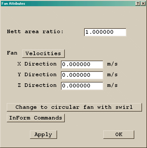
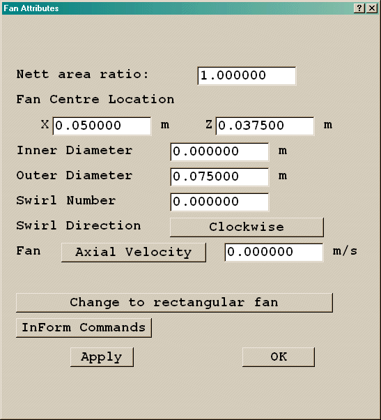
Image: INTERNAL FAN DIALOGS
InForm Commands
This leads to a dialog from which a selection of InForm commands can be attached to this object. It is described InForm Commands below.
Single Phase, Multi-phase, Radiative Heat Loss, Internal Outlet, InForm
An outlet (also referred to as an OPENING in Flair) is a region of fixed pressure. Outlets can only be attached to area objects. The flow direction is actually unspecified, and depends on local pressure differences, although usually the flow will be out of the domain.
The default geometry for an outlet is public\default\box.dat, the default colour is light blue (colour 214), and the default opaqueness is 50, representing a transparent blue cuboid.
The Outlet attributes dialog box is shown below:
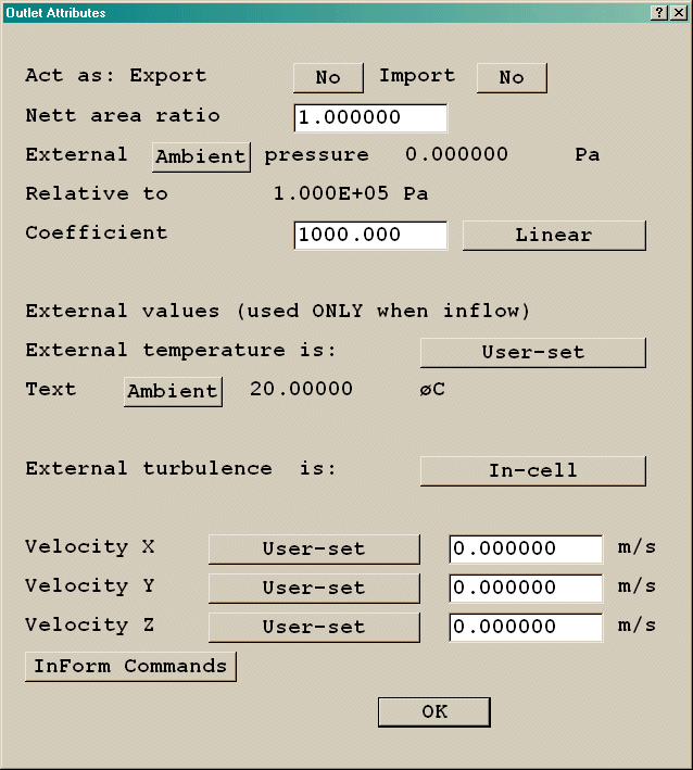
Image: SINGLE PHASE OUTLET ATTRIBUTES
Acts as: Export / Import allows the outlet object to behave as a Transfer Object. When Export is activated, an input box for the export file name appears. The default is the current object name. At the end of the Solver run, the named file is created. It will contain the mass flows and other variables for each cell covered by the object.
If Import is activated, the remaining attributes are hidden, as the flow conditions will be read from a file. The file name can either be entered into the input box, or searched for with a file browser. The default is also the current object name.
The Nett area ratio sets the ratio between the area actually available for flow, sometimes called the effective area, and the area used in the model. It is used to deduce the inflow velocity when there is inflow and the external velocity is set to 'deduced'.
The Coefficient controls how closely the internal pressure matches the set external pressure. When the Coefficient is set to 'Linear', the mass flow rate through the outlet is linearly proportional to the pressure difference.
m" = ρ*vel = ΔP*Coef
When it is set to 'Quadratic ', the mass flow is proportional to the square root of the pressure difference. This is appropriate for a known loss coefficient KL.
ΔP = 0.5*KL*ρ*vel2 -> m" = ρ*vel = ((2*ρ/KL)*ΔP)0.5
The loss coefficient KL should be entered directly into the 'Coefficient' input box.
The external pressure is set relative to a fixed reference pressure. The reference pressure is set from the ' Main Menu - Properties' panel. The external pressure can be the ambient pressure set on the Main Menu, Properties panel, or any user-set value.
In order to specify a stagnation / total pressure the user should specify the desired stagnation / total pressure value, relative to the reference pressure, as the external pressure. This pressure is then set with a coefficient KL of 1.0. Furthermore, the velocity component perpendicular to the outlet should be set to Deduced (see below), ideally with a good initial estimate of the anticipated final value.
The temperature and velocity values are only used if flow should enter. In cells where flow is out of the domain, the settings of external values will be ignored. They will only be used in those cells where fluid is entering the domain.
The available settings are In-cell and User-set. For velocity there is an extra option, Deduced.
The IPSA outlet dialog box is shown below:
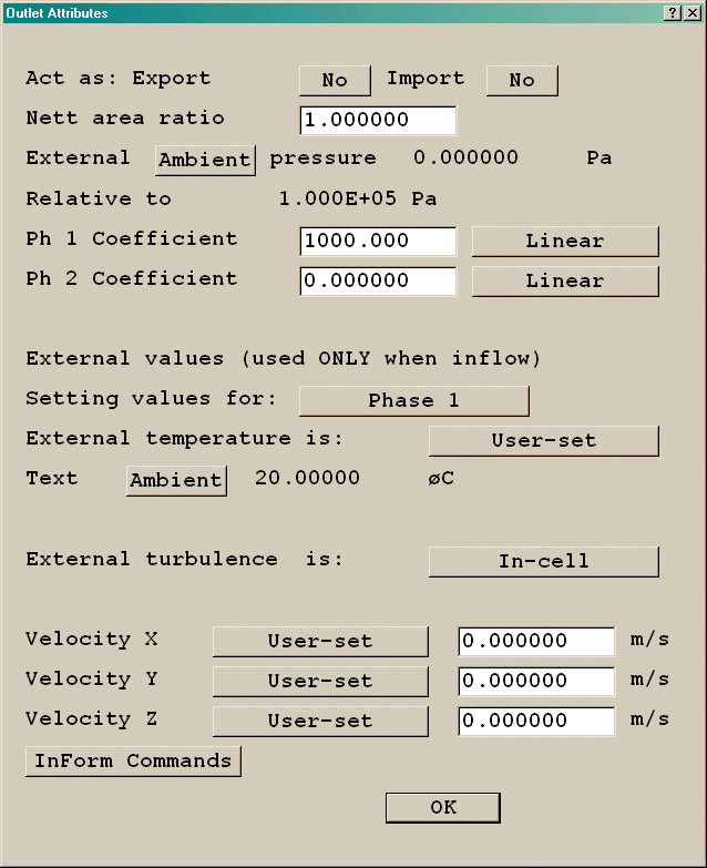
Image: MULTI-PHASE OUTLET ATTRIBUTES
By default, both phases are allowed to pass through. The coefficients for the two phases should ideally be in the ratio of the phase densities. The default settings are appropriate for phase 1 density of the order of 1.0, and phase 2 density of the order 1000.
If only one phase is to be allowed to pass through, the coefficient of the other phase should be set to zero, to block its passage.
The 'Setting values for' button sets which phase the external values are being set for.
If the Lagrangian Particle tracker GENTRA is active, Outlets can be set to act as particle exits.
If the IMMERSOL radiation model is active, the outlet can be allowed to exchange heat by radiation with the surroundings. If the External radiative link is set to Yes, the temperature of the surroundings, Texternal, can be set. The heat flux from the outlet will then be:
Q" = σ (Text4 - Tp4) (W/m2)
where σ is the Stefan-Boltzmann constant.
If the outlet is internal to the domain, an extra button appears on the dialog box, labeled Object side. The settings for this are Low or High, and they indicate whether the outlet is to appear on the low-co-ordinate face or high-co-ordinate face of the object.
When inside the domain, outlet objects are usually located on the face of a BLOCKAGE. They represent the inflow to some ducting that is not being modeled.
--------
| |
---->|Blockage|---->
| |
--------
L H L H
---------> X, Y or Z
If the setting is 'LOW', as on the left side above, the outlet acts on the smaller-coordinate side of the inlet. If the setting is 'HIGH',as on the right side above, the outlet acts on the larger-coordinate side.
If the setting is HIGH on the left side or LOW on the right side, the outlet acts inside the blockage and nothing happens at all.
This leads to a dialog from which a selection of InForm commands can be attached to this object. It is described in InForm Commands below.
An Angled-out is a region of fixed pressure. The region of influence is the part of the surface of any blockage object(s) enclosed by the angled-out object. The angled-out object itself must be a 3D volume. The flow direction is actually unspecified, and depends on local pressure differences, although usually the flow will be out of the domain.
The default geometry for an angled-out s public\default\box.dat, the default colour is light blue (colour 214), and the default opaqueness is 50, representing a transparent blue cuboid.
The angled-out object may intersect a blockage, as shown here:
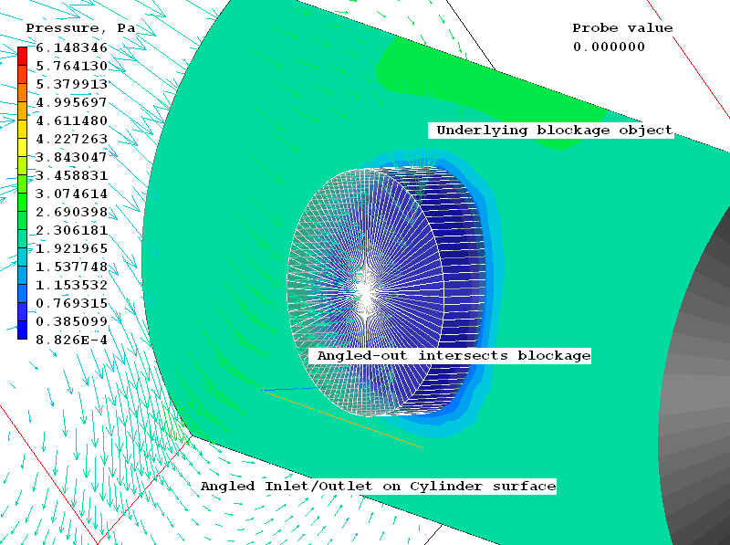
IMAGE: Angled-out intersects blockage
It may also completely surround a blockage, as shown here:
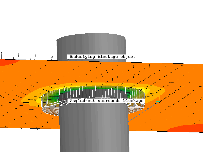
IMAGE: Angled-out surrounds blockage
Its area of influence cannot lie on the domain edge, as it must intersect a blockage.
The attributes of the Angled-out object are as those of the 'normal' outlet, with the addition of 'Normal velocity' to the methods of specifying the external velocity. This sets the velocity normal to the surface of the underlying blockage, should there be an inflow in any affected cell.
The function of the WIND object is to provide boundary conditions representing the atmospheric boundary layer due to the wind at all faces of the domain in a self-consistent manner. The following conditions are applied:
The wind direction and 'up' direction set by the user control which condition is applied to which domain face.
The velocity profile to be used can be:
For a logarithmic profile, the velocity is computed from expressions compatible with the fully-rough wall function, described here. The velocity is calculated from:
U/U* = ln((z-d)/zo )/ κ
where the total friction velocity U* is given by:
U*= Ur κ/ln((zr-d)/zo)
Z is the local height above the ground, zr is a reference height, Ur is the wind velocity at the reference height, d is the boundary layer zero plane displacement height, zo is the roughness height and κ is Von Karman's constant (=0.41).
The above two expressions simplify to give:
U/Ur = ln((z-d)/(zr-d))
For a power-law profile, the velocity is computed from:
U/Ur= (z/zr)α
where Ur and zr are the reference velocity and height, and α is the power-law exponent.
In either case the turbulence quantities are set to:
k = U*2/√(CμCd); ε= U*3/(κ*z)
or, for the k-omega model:
k = U*2/√(CμCd); ω= U*/(κ√(CμCd)z)
For tabular profiles, two files need to be specified. One contains the variation of velocity with height, and one the variation of turbulent kinetic energy (k) with height. The files are ASCII free format. The first line is a header, often the titles of the columns of data. The following lines contain pairs of values with a space or comma (,) as separators, representing height and U or k respectively. The two files do not need to contain data at the same heights, or the same number of data points.
An Excel .csv file is a good example. The first few lines of a typical file are shown:
Distance,UIN
 0.000000E+00, 2.811892E+00
 9.999998E+00, 2.851801E+00
 2.000000E+01, 2.891711E+00
 2.999999E+01, 2.931620E+00
 3.999999E+01, 2.971529E+00
The inlet value of ε is now computed from:
ε = Cd k3/2/(κz)or for the k-omega model the inlet value of omega is computed from:
ω = √k/(κ(CμCd)0.25z)
If the tables do not contain enough data points to cover the entire height of the domain, then at heights below the first point in the table the first value will be used, and at heights above the last point in the table the last value will be used.
It is the user's responsibility to ensure that the velocity and turbulence values in the data files are correct, and also to ensure that the roughness height z0 is set to a value such that the shear stress at the ground produced by the fully-rough wall functions is compatible with that implied by the tabulated profiles.
The height above the ground, z, is measured from the first open cell in each column of cells. This allows the profile to follow the terrain imposed by a blockage.
For Power-law and tabular velocity profiles, the inlet temperature profile is assumed constant. For the default logarithmic velocity profile the temperature profile can be obtained using one of the Pasquill stability classes and a Monin-Obukhov length. A full description of these is given here.
Dialogs, Weather Data, Radiative heat loss, Transient operation, Initialisation, GENTRA, Wind Amplification factor
The initial WIND attributes dialog is shown here:
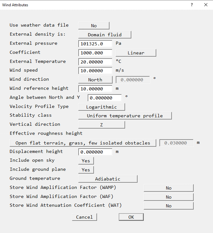
IMAGE: WIND Dialog
The image shown is with the Energy equation active. For iso-thermal cases (i.e. Energy equation is OFF) the items relating to temperature are not displayed.
In transient cases, multiple WIND objects are allowed on the basis that their start- and end-times do not overlap. This gives the possibility to allow the wind direction and / or speed to change with time. However, if a weather file is being used, a single WIND object will pass all the required time-varying data to the solver.
The items on the dialog are as follows:
Use weather data file. When set to No, as shown above, the user must supply all the required input data as set out below. When set to Yes, the input data are taken from an EnergyPlus EPW weather data file. The method for doing this is described in the section 'Loading a Weather Data File' below. The data in the weather file can also be used by a SUN object to supply the solar heating load. WIND and SUN always use the same weather file, and will use data for the same date and time. If tabular profiles have been selected, the option to use a weather file is not shown.
External density. The external density is used to calculate the mass inflow. It can be taken to be the same as the domain material density, or set to a user-specified value. If the domain density is a function of pressure (and/or temperature), the External pressure (and/or External temperature) will be used to evaluate it.
External pressure. This sets the pressure outside the domain. It is taken to be the same at all open faces. It may be used to calculate the inlet density. The external pressure is the atmospheric pressure at the edges of the domain. The reference pressure (PRESS0) is reset to this value. The reference pressure can be seen on the 'Main Menu - Properties' panel. The Ambient pressure seen on the 'Main Menu - Properties' panel is set to zero.
When a weather file is in use, the external pressure is taken from the weather file.
On the downwind, fixed pressure, faces, the pressure is set to zero relative to the reference pressure, which has been automatically set to the external pressure.
Coefficient. This controls how closely the internal pressure at the down stream boundaries (and upper boundary if Sky is active) approaches the set external pressure. When set to Linear, the mass flow through the pressure boundaries is a linear function of pressure difference. A fairly large value of the order of 1000 will keep the internal pressure very close to the external, suppressing any internal pressure gradients at the boundaries. When set to Quadratic, the coefficient represents a loss in dynamic head across the boundary. The mass flow is proportional to the square root of pressure difference. A small number should be used to reduce the pressure loss. See the entry on Coefficient in the Outlet object description below for more details.
External Temperature. This sets the ambient temperature outside the domain. It is specified as the external value at all the faces, and may be used to calculate the inlet density. The Ambient temperature seen on the ' Main Menu - Properties' panel is reset to the external temperature. This, together with resetting the reference pressure to the external pressure, enables the reference density used for buoyancy to be set equal to the density at the external pressure and temperature.
When a weather file is in use, the external temperature is taken from the weather file.
Wind speed. This sets the absolute value of the wind velocity in m/s at the reference height. When a weather file is in use, the value is taken from the weather file. This item is not shown if tabular profiles have been selected.
Wind direction. This sets the direction that the wind is blowing from. There are sixteen pre-set directions of North, North-North-East, North-East, East-North-East, East, East-South-East, South-East, South-South-East, South, South-South-West, South-West, West-South-West, West, West-North-West , North-West and North-North-West.
To specify any other direction, select 'User' and enter the required angle in degrees, relative to North. A value of zero means that the wind is blowing from due North. The angle increases clockwise to 90 for East, 180 for South and 270 for West. Any value in the range -360.0 to 360.0 is valid. When a weather file is in use, the direction is set to File, and the value is taken from the weather file.
The wind direction is always relative to North.
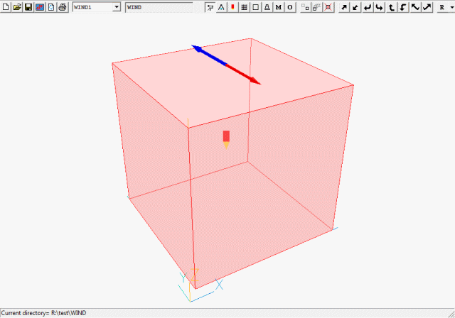
IMAGE: WIND object representation
The blue arrow points to North, and the red arrow shows the direction the wind is blowing from, in this case from the North.
Wind Reference height. This sets the height at which the Wind Speed is specified. This item is not shown if tabular profiles have been selected.
Angle between Y (or X or Z) axis and North. This, and the Vertical direction determine the orientation of the domain with respect to North. With the angle set to zero,
In the example below, increasing the angle will rotate the North-facing axis (i.e. Y) clockwise when looking down along the vertical axis (i.e. Z):
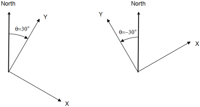
This allows the domain to be oriented conveniently with respect to a building or group of buildings.
Velocity Profile type. The boundary layer velocity profile can be a logarithmic or power-law function of height above the ground, or read from tables as described above in the Overview section. If a weather file has been activated, only the logarithmic and power-law options can be used. The height is measured from the first open cell.
Stability class. The thermal stability class can be selected from:
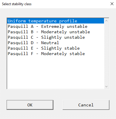
The classes are defined in the table below:
| Wind speed (m/s) | Daytime Insolation | Night time conditions | |||
| Strong | Moderate | Slight | Thin overcast >= 4/8 low cloud | <=3/8 cloud | |
| 2 | A | A-B | B | - | F |
| 2-3 | A-B | B | C | E | E |
| 3-5 | B | B-C | C | D | D |
| 5-6 | C | C-D | D | D | D |
| >6 | C | D | D | D | D |
Monin-Obukhov length.
If one of the Pasquill classes is selected, another line appears for the Monin-Obukhov length:
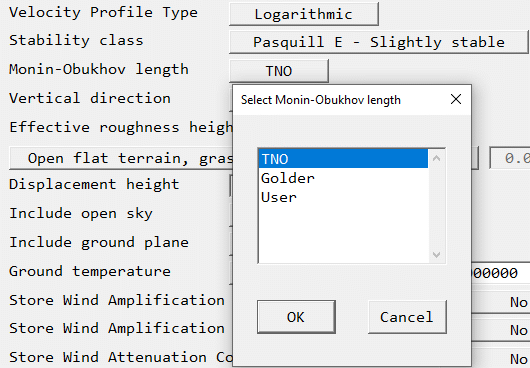
Please see the full description for further explanations.
Vertical direction. This controls which axis will be pointing up. The options are Z, Y or X. It is not possible to make the vertical axis point downwards.
Effective roughness height. This sets the roughness height at the edge of the domain. Typical values are given below. Values can be selected from a list, or a user-set value can be entered.
| Surface type | Roughness height zo (m) | Power-law exponent α |
| Open sea | 0.0002 | 0.16 |
| Open flat terrain, grass, few isolated obstacles | 0.03 | 0.13 |
| Low crops, occasional large obstacles | 0.10 | 0.16 |
| High crops, scattered obstacles | 0.25 | 0.19 |
| Parkland, bushes, numerous obstacles | 0.50 | 0.21 |
| Suburb, forest, regular large obstacle coverage | 0.50 to 1.0 | 0.21 to 0.24 |
The default roughness height is 0.03 - Open flat terrain, grass, few isolated obstacles.
It is advisable to set the roughness height of the object used to represent the ground to the same value, and to set the wall-function type to 'Fully-rough' to ensure that the wind profiles are maintained within the domain. This value should not be greater than the height of the first cell-centre above the ground.
Displacement height. The displacement height is the distance above the ground at which zero wind speed is achieved as a result of flow obstacles such as trees or buildings. Often the displacement height is zero, but for flow over an array of densely packed objects (e.g. a forest, cropland or buildings), an offset in height is introduced into the log law to allow for the upward displacement of the flow by the surface objects.
This displacement height d is usually estimated as 2/3 of the average height of the obstacles.
The displacement height d is a positive quantity, although the user can set d=-roughness height to use wall functions that are consistent with the inlet wind profiles proposed by Richards & Hoxey (1993)11, which are often used in wind-engineering simulations.
Include open sky. When set to No, the upper boundary is treated as a frictionless impermeable lid. When set to Yes, the upper boundary is treated as a fixed pressure boundary. The external pressure, pressure coefficient and temperature are the same as at the down wind boundaries. The free stream velocities and turbulence quantities are calculated from the boundary layer formula at that height above the ground. In addition, the diffusive link between the top cell and the free stream value is activated. This helps to preserve the boundary layer profile.
Include ground plane. When set to No, the ground plane is left as a frictionless adiabatic surface. It is up to the user to provide an appropriate boundary condition, by using a PLATE object to represent flat terrain, a BLOCKAGE (or in Flair a TERRAIN) object to represent undulating terrain or a combination of these. The 'Wall function law' for these objects should be set to 'Fully rough' (default for TERRAIN), and the roughness height set to the same value as that used for the inlet profiles. Note this should be set as the wall function law for the terrain object(s) only - the default wall function set in the Main Menu - Sources panel should be left as 'Log-Law'.
When set to Yes, a ground plane with the appropriate wall function and roughness height settings will be created to cover the whole of the bottom face of the domain.
Surface emissivity If the IMMERSOL radiation model is active, the emissivity of the surface can be set. For most substances absorption is 0.5 or greater; bricks, weathered steel and marble can be up to 0.9. The exceptions are polished metal surfaces -typically .1-.2.
Solar absorption factor. When the ground plane is included, the 'Solar absorption factor' determines how much of the incident solar radiation is absorbed. This is a non-physical factor which can be used to diminish the amount of solar energy (specified with the Sun object) which is absorbed by the ground surface. This can be used as a crude representation of diurnal effects when the Sun object is used in the context of a steady model.
Ground Temperature. When the ground plane is included, the ground surface can be adiabatic or fixed surface temperature. This temperature is set by the user. If a weather file is in use, the value is taken from the weather file. If other thermal conditions are required, the ground plane can be turned off, and a PLATE object used instead.
If the IMMERSOL radiation model is active, the domain boundaries can be allowed to exchange heat by radiation with the surroundings. If the External radiative link is set to Yes, the temperature of the surroundings, Texternal, can be set. The heat flux from the wind profile boundary will then be:
Q" = σ (Text4 - Tp4) (W/m2)
If the Lagrangian Particle tracker GENTRA is active, the domain boundaries will act as particle exits by default. This can be switched off.
When a weather data file is not being used, the operating time of the WIND object can be set as for most other objects. A number of WIND objects can be created with consecutive start and end times, each with different flow conditions. This way the time variation of wind speed and direction can be accommodated.
When a weather data file is being used, the situation is simpler. The date and time chosen represent the time at the start of the calculation. The time-varying data is extracted from the weather file and is passed to the Earth solver automatically. Only one WIND object is needed.
If the initial values for the velocities are all left at their default values of 1E-10m/s, the WIND object will impose initial conditions based on the chosen boundary layer formula, shown below for the WIND_PROFILE object.
If the initial values of the turbulence quantities KE and EP are left at their default values of 1E-10, the WIND object will impose initial conditions based on the logarithmic profile.
The values used by the WIND object are echoed to the RESULT file, as in this example:
************************************************************
Wind profile data
-----------------
Up direction Z
Inlet density 1.204938E+00 kg/m^3
Reference height 1.000000E+01 m
Roughness height 1.000000E-01 m
Profile type - Logarithmic Law
Pressure coeff at outflow boundaries 1.000000E+03
Wind direction 9.000000E+01°
Wind speed 1.000000E+01 m/s
Air temperature 2.000000E+01°C
************************************************************
When 'Store Wind Amplification Factor WAMP' is set to 'Yes', an additional 3D variable called WAMP will be STOREd, and the solver will fill it with values of the local air velocity divided by the wind-profile speed at the set reference height, often 1.5m.
When 'Store Wind Amplification Factor WAF' is set to 'Yes', an additional 3D variable called WAF will be STOREd, and the solver will fill it with values of the local air velocity divided by the wind-profile speed at the local height. In the absence of buildings, WAF should be 1.0 everywhere. It is an indicator of the local change in wind speed caused by the buildings.
The following restrictions apply to the wind object:
The WIND object always fills the entire domain. Once the user is certain that it is oriented correctly, it can safely be hidden, or made wire-frame so that it does not obscure the objects within the domain. An alternative is to make it not selectable, so that the internal objects can be picked from the screen. The WIND object can always be selected from the Object Management Dialog
Dialogs, Weather Data, Transient operation, Absorption of solar radiation by objects, Additional output, Limitations
The SUN object applies the direct and diffuse solar radiation heat load to objects within the domain, taking into account:
Solar radiation perpendicular to the sun's rays at the top of the earth's atmosphere has an annual mean irradiance of approximately 1370 W/m2, with a seasonal variance of around +/- 3.5W/m2. In passing through the atmosphere, part of this energy is absorbed by the atmosphere, part is scattered by the atmosphere - some back into space and some to the earth (the diffuse 'sky' radiation), and the remainder (direct radiation) is transmitted through the atmosphere unchanged.
There are many sources available from which values of the direct and diffuse radiation may be obtained. One such source is the collection of weather data files from the U.S Department of Energy, freely available as part of the EnergyPlus Energy Simulation Software. Weather data for more than 2100 locations are now available in EnergyPlus weather format - 1042 locations in the USA, 71 locations in Canada, and more than 1000 locations in 100 other countries throughout the world. The weather data are arranged by World Meteorological Organization region and Country.
The sun object can use these weather data files directly to obtain the direct and diffuse solar radiation at a particular date and time of day. The WIND object can also read the weather data file to obtain the wind speed and direction, and the temperature of the air and ground.
The default SUN dialog is shown here.
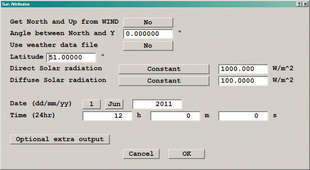
IMAGE: SUN dialog
Get North and Up from WIND. When set to No, the user must specify the orientation of the domain relative to North. When set to Yes, the orientation is shared with the (first if more than one) WIND object (which must have been created already). When shared with WIND, the input box on the SUN dialog is grayed out, and any change in domain orientation must be made on the WIND dialog. This ensures that the SUN and WIND are oriented identically eliminating a potential source of error.
Angle between Y axis and North. This works in the same way as for the WIND object. It allows the domain to be oriented conveniently with respect to a building or group of buildings.
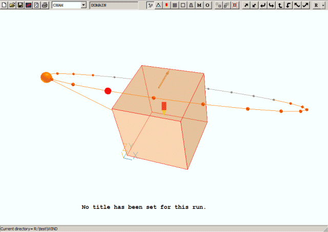
IMAGE: SUN Object
The orange arrow points North. When 'Get NORTH and UP form WIND' is set to Yes, the orange arrow is not drawn as it is then the same as the WIND's blue arrow.
In the example below, increasing the angle will rotate the North-facing axis (i.e. Y) clockwise when looking down along the vertical axis (i.e. Z):
Use weather data file. When set to No, as shown above, the user must supply all the required input data as set out below. When set to Yes, the input data are taken from an EnergyPlus EPW weather data file. The method for doing this is described in the section 'Loading a Weather Data File'. The data in the weather file can also be used by a WIND object to supply the inflow/outflow conditions at the domain boundaries. SUN and WIND always use the same weather file, and will use data for the same date and time.
Latitude. This sets the latitude of the location. The Equator is at 0 degrees, the Northern hemisphere is 0 to 90 (at the North pole), and the Southern is 0 to -90 (at the South pole). If a weather file is in use, this is set to the value read from the weather file.
Direct Solar radiation. This sets the incident solar radiation in W/m2. In the EnergyPlus data sets this is referred to as the Extraterrestrial Direct Normal Radiation. If a weather file is in use, this is set to File and the value is taken from the weather file.
If a weather file is not in use, it can be set to Constant or From solar altitude. In the latter case the direct solar radiation is obtained from polynomial fits to tables A2.24 (direct) and A2.25 (diffuse) of The CIBSE Guide, Volume A Design Data. These give the following values in W/m2:
| Solar Altitude (degrees) |
Direct Radiation Normal to Sun (W/m2) |
Diffuse Radiation (W/m2) | |
| Clear | Cloudy | ||
| 5 | 210 | 25 | 25 |
| 10 | 390 | 40 | 50 |
| 20 | 620 | 65 | 100 |
| 25 | 690 | 70 | 125 |
| 30 | 740 | 75 | 150 |
| 35 | 780 | 80 | 175 |
| 40 | 815 | 85 | 200 |
| 45 | 840 | 90 | 225 |
| 50 | 860 | 95 | 250 |
| 60 | 895 | 100 | 300 |
| 70 | 910 | 105 | 355 |
| 80 | 920 | 110 | 405 |
| 90 | 930 | 115 | 455 |
The solar altitude is obtained from the sun direction vector as calculated either at the start of the run, or at the start of each step in a transient.
Diffuse Solar radiation. This sets the diffuse solar radiation in W/m2. If a weather file is in use, this is set to File and the value is taken from the weather file. If a weather file is not in use, it can be set to Constant or From solar altitude, in which case values are interpolated from the table above, with the solar altitude calculated from the latitude, date and time of day. The further setting Clear sky or Cloudy sky determines which column to use.
Date. This sets the date (Day, Month, Year) at which the sun position is calculated. Strictly only the day and month are important. If a weather file is in use, this entry is taken from the weather file.
Time. This sets the time of day (using the 24 hour clock) at which the sun position is calculated. The time here is in effect local time, not taking any daylight-saving into account. At 12:00 (noon) the sun is at its highest position. If a weather file is in use, this entry is taken from the weather file.
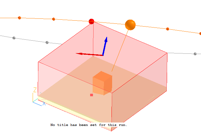
In the image above, the large orange ball marks the sun position at the current time of day. The small orange balls denote the sun position on the hour during the day, and the grey balls at night when the sun is below the horizon. The red ball denotes the sun position at midday. The orange line drawn from the current sun position to the middle of the ground plane shows the direction of the sun's rays.
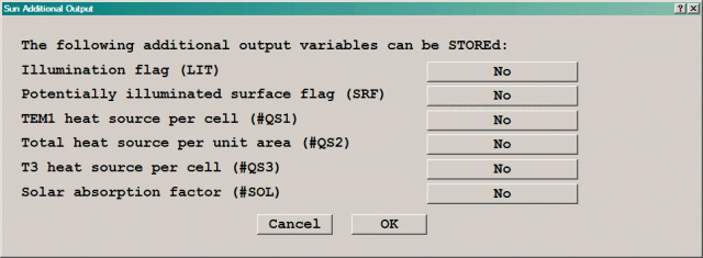
There are several optional settings which can help to show how the model is working. These are activated from the 'Optional extra output' dialog:
Consider the following simple example, in which the sun is shining from the front to the back.
The following 3D variables can be stored:

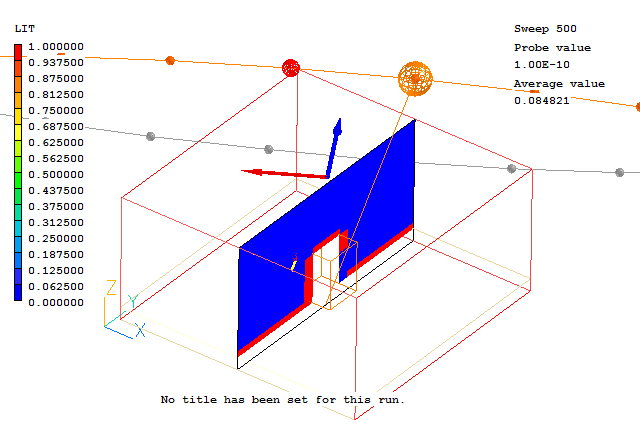
There is one cell near the top of the block which appears illuminated, but is on the back face of the central block. The centre of this cell can still see the sun.
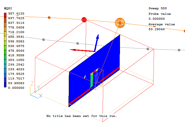
In this image the suspicious cell can be seen to have only the diffuse heat source, as the face is pointing away from the sun.
When plotting these variables in the Viewer it is best to turn the contour averaging off, otherwise the averaging process will introduce values of SRF and LIT between 0 and 1 which do not exist. The heat sources only exist in a single layer of cells, so the averaging will appear to dilute them.
In a transient case, the time that should be set is the time at the start of the calculation. At each time step, the position of the sun will be adjusted, and the shading and resulting heat sources recalculated.
If a weather data file is in use, the radiative loads at each time in the data file are passed to the Earth solver. The solver will perform a linear interpolation between these values to find the value at the current calculation time.
If a weather file is not in use, the solar radiation can either be a constant, or can be derived from the solar altitude as described above. The solar altitude will be automatically updated for each time step.
Absorption of Solar Radiation by Objects
When the SUN object is active, an extra input appears on the dialogs of BLOCKAGE, PLATE and THIN PLATE objects. This sets the amount of incident solar radiation absorbed by that object. The default absorption factor is 1.0 - i.e. all the heat is absorbed by the object. For most substances absorption is 0.5 or greater; bricks, weathered steel and marble can be up to 0.9. The exceptions are polished metal surfaces -typically .1-.2.
For participating blockages the solar energy is deposited in the outer-most layer of cells in the blockage. From there, the heat can be conducted away into the center of the blockage, as well as being convected and radiated away from the surface.
For non-participating blockages (.i.e. those using the 198 or 199 materials) and for plates, the solar energy is deposited in the layer of fluid cells adjacent to the object.
The settings in use by the sun object are echoed into the RESULT file by the solver, as shown in this example:
************************************************************
Solar Heating data
------------------
Latitude 51.00°
Time of day JUN 01 15:00:00 2011
Constant direct solar heating 5.000000E+02 W/m^2
Constant diffuse solar heating 1.000000E+02 W/m^2
************************************************************
************************************************************
Solar altitude: 4.400269E+01°
Direct solar radiation: 5.000000E+02 W/m^2
Diffuse solar radiation: 1.000000E+02 W/m^2
************************************************************
The shading calculation is very dependent on there being enough grid to resolve sufficient detail of the geometry. If the grid is too coarse the illumination and resulting heat sources will be inaccurate.
The shading algorithm only works with Z as the UP direction.
The SUN object always fills the entire domain. Once the user is certain that it is oriented correctly, it can safely be hidden, or made wire-frame so that it does not obscure the objects within the domain. An alternative is to make it not selectable, so that the internal objects can be picked from the screen. The SUN object can always be selected from the Object Management Dialog.
The Pressure Relief object is used to create a fixed-pressure point, usually in an enclosed domain. It does not affect the grid - the cell whose centre is nearest the position is used as the fixed-pressure cell.
The only attributes are pressure coefficient and value. Value is the pressure to be fixed, relative to the reference pressure set in the Properties panel of the Main Menu. Coefficient fixes how closely the pressure in the domain matches the set value. A coefficient of 1000 is often found to work well.
Note: The pressure-relief object does not affect the grid. The size of the object is adjusted on exit from VR to cover the cell nearest the origin of the object.
The default geometry for a Pressure Relief object is public\default\cubet.dat, a transparent grey cuboid
The Heat_source object is used to create an area or volume over which heat is released. It differs from a Blockage in that no material is associated with this object.
Object Attributes
This object type is used to model the interaction between the wind and forested areas, as well with other types of tree or plant canopy, such as for example urban plantings of avenues or clumps of trees. From an aerodynamic perspective, the main impact of vegetation on the environment is the reduction in air velocity due to drag forces, and the additional turbulence levels produced by the canopy elements.
These effects are represented by a porous-media approach based on superficial velocities where momentum sinks and turbulence sources are applied to a block of cells chosen to represent the tree canopy. Consequently, the influence of vegetation on the turbulent flow fields is modeled by the inclusion of drag forces in the momentum equations, and additional source terms in the transport equations for the turbulent kinetic energy k and its dissipation rate ε. These drag forces are responsible for the deceleration of the wind flow inside the plant canopy, and the additional turbulence source terms account for turbulence production and accelerated turbulence dissipation within the canopy ( see Finnigan (2000)1 ).
The foliage object must be a 3D volume. The default geometry is public\default\box.dat, the default colour is light green (colour 125) and the default opaqueness is 50, depicting a transparent green cube. Any 3D geometry of the user's choice can be used instead.
Momentum Sink due to Form Drag
The flow resistance due to turbulent flow through the plant canopy is represented by introducing the following sink term into the momentum equations:
Sd,i = -ρ Cd α(z) |U|ui
where ρ is the fluid density, Cd is the drag coefficient, α(z) is the leaf-area density (LAD) perpendicular to the flow direction in m2/m3, z is the vertical space coordinate, |U| is the magnitude of the superficial velocity vector, and ui is the superficial value of the Cartesian velocity in the direction i.
The default PHOENICS model uses a constant effective drag coefficient Cd and a constant effective leaf- area density α. The vegetation density is characterised by the leaf-area density and its integral value, the leaf area index (LAI), which is defined by:
LAI = ∫0hα(z)dz
where h is the average height of the canopy. For computational convenience a vertically constant leaf area density is assumed, which can be computed from the leaf area index and canopy height via:
α = LAI / h
An alternative is to allow the leaf area density to vary with height. The variation of α with height is read from a file.
Turbulence
The turbulent interaction between the airflow and the plant canopy is simulated by including the following additional source terms in the transport equations for k and ε:
Sk = ρCdα(z)(βp|U|3 - βd|U|k)
and
Sε = ρCdα(z)(C4εβp|U|3 ε/k - C5εβ d|U|ε)
where βp, βd, C4ε and C5ε are empirical constants. The constant βp represents the fraction of mean-flow kinetic energy converted to wake- generated k by canopy drag, and βd is the fraction of k dissipated by short-circuiting of the Kolmogorov energy cascade. Therefore, the source terms in these equations account for wake production, whereas the sink terms account for the spectral short cut associated with the production of turbulence in the wakes behind the individual canopy elements (branches, leaves, etc).
As shown in the table below, there is little consensus about their recommended values, which reflects the fact that different values are needed to match different sets of measured data. The default values used in the PHOENICS implementation are those of Green3.
| Model | βp | βd | C4ε | C5ε |
| Svensson et al (1990)2 | 1.0 | 0.0 | 1.95 | 0.0 |
| Green (1992)3 | 1.0 | 4.0 | 1.5 | 1.5 |
| Liu et al (1998)4 | 1.0 | 4.0 | 1.5 | 0.6 |
| Sanz (2003)5 | 1.0 | 5.1 | 0.9 | 0.9 |
| Krzikalla (2005)6 | 0.0 | 4.0 | 0.0 | 1.075 |
| Lopes da Costa (2007)7 | 0.17 | 3.37 | 0.9 | 0.9 |
Note that the Lopes da Costa model can only be used with the standard K-ε model, as it also adjusts the basic model constants. It changes CµCd from the usual 0.09 to 0.033, and the turbulent Prandtl/Schmidt Number for ε from 1.84 to 1.3. Because of this, the Lopes model can only be selected if a) the turbulence model is KEMODL, and b) it is the first foliage object.
Object Attributes
The foliage attributes dialog with default settings is shown below:
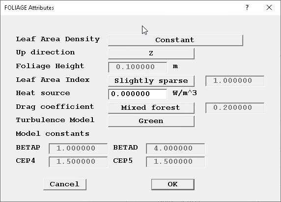
By default, this is taken to be constant with height, and deduced from the foliage height and Leaf Area Index as indicated above.
The alternative is to allow the Leaf Area Density to vary with height. In this case, the variation of LAD with height is held in an ASCII file. There are two options for how the height is defined.
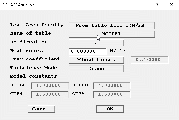
The first, illustrated in the image above, is for the height to be normalised by the forest height i.e. the LAD is a function of h/FH where FH is the vertical size of the foliage object. The second option is for the height to be the actual height in metres. Note that the height used is the height above the origin of the foliage object.
Click on NOTSET to open a file browser to find the required file. The file should contain two columns of values in free format. The first is vertical position, h/FH or h, the second LAD at that height. The solver will interpolate in the table file to find the LAD at each grid plane. A typical file might look like this:
 Y/FH        LAD
0.00        0.0
0.268293    0.0484006
0.361419    1.09652
0.665188    0.178581
1.0         0.00333797
This sets the vertical coordinate. When Leaf Area Density is constant, the foliage height is taken to be the object dimension in this direction. When Leaf Area Density is taken from a file, the interpolation in the file is performed in this direction.
The options provided for Leaf Area Index are taken from Huang at al (2008)8 and are shown below.
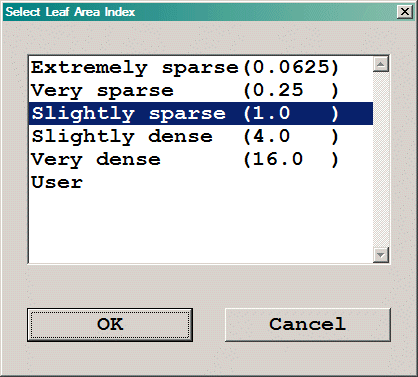
Selecting 'User' allows any required value to be entered into the input box.
The values of drag coefficient Cd can be expected to show a large variation with respect to type of vegetation, foliage density, etc. Information concerning the drag coefficient of different types of trees and plants can be found in the literature (see for example Zeng & Takahashi (2000)9 and Van Renterghem & Bottledooren (2008)10 ). Typically, values for individual deciduous trees range from 0.15 to 0.25, and a value of 0.2 is commonly used in numerical studies of wind flow through forests. Measured drag coefficients for single-row deciduous "windbreak" species are reported to be near 0.5, whereas coniferous types of trees are characterised by somewhat larger values in the range 0.6 to 1.2. This is reflected in the values provided for the Drag Coefficient.
As for LAI, selecting 'User' allows any value to be entered.
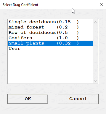
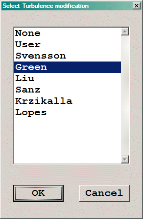
Selecting 'None' switches off the addition source / sink terms described above. Selecting 'User' allows any desired values to be input for the empirical constants. For the remainder, the constants are set as shown in the table above.
If the Energy Equation is active, an extra input box (shown above) appears. This allows the cooling power of the vegetation due to evaporation to be specified. A typical cooling power is 250 W/m3. This is multiplied by the Leaf Area Density internally. If the vegetation is absorbing heat, a negative value should be specified.
In Flair, if the humidity model is active an additional input box appears for the moisture source due to evaporation from the plants. The source set should be in kg/m3/s. This source is then multiplied by the Leaf Area Density internally. A typical moisture release rate might be 810gm/m3/day which is 9.375*10-6kg/m3/s.
The cooling power and humidity source values are taken from Zhang (2019)12. More values for specific species can be found in Mo et al (2007)13.
If any scalar equations are being solved, an additional pair of lines appear:
Scalar source
This brings up a list of all scalar equations currently allowed to have sources.
Value
The value of the source in kg/m3/s can be entered here. If the vegetation is absorbing the scalar, a negative value should be set. This source will also be multiplied by the Leaf Area Density internally.
This allows any user-defined PATCH to be attached to an object. The Lecture on Boundary Conditions, and the Encyclopaedia entries on PATCH, COVAL and TYPE give more details on what settings to make. The default geometry is public\default\box.dat, and the default colour is khaki (colour 56) representing a khaki cuboid.
Image: UNIVERSAL OBJECT ATTRIBUTES
To create a new patch, click on New, and enter a name, up to seven characters long. Click on Apply to create the patch. Click on Type, and enter the patch type, e.g. HIGH or NORTH. Finally, click on the Coefficient and/or Value slots required, and enter the values.
As many Patches as required can be attached to a single object. Clicking on PATCH number will cycle through the available Patches. The > (and <) symbol next to Variable scrolls through the list of available variables, if there are more than five.
The object can be an area or a volume.
Note that if the object type is changed from user_defined to some other type, a dialog will appear offering to delete any patches declared. This should be done, otherwise they will remain in the Q1 file and may introduce unwanted sources / sinks.
A ROTOR object represents a zone of rotating co-ordinates in a cylindrical-polar grid. Within the scope of this object, the grid is rotating about the Z axis with a set speed. Here, additional sources are added to the X- and Y-direction velocities to account for the centrifugal and Coriolis forces associated with the rotation. At the boundaries of the rotating zone, frame transformations have to be applied to convection and diffusion terms.
Note: A ROTOR object cannot be used in a Cartesian or BFC system.
Any BLOCKAGE objects falling within the scope of the ROTOR object will rotate with the rotor. A typical use for this object type is to model a rotating fan or impeller.
The advantage of this over the whole-domain rotating co-ordinates activated from the Sources panel is that the objects within the ROTOR can move relative to other stationary objects.
Image: ROTOR Object dialog (for transient case)
The above image shows the ROTOR Attributes dialog for a transient case. It is also possible to use ROTOR objects in steady-state. In steady-state, the equations inside and outside the ROTOR are still solved in their respective frames of reference, with appropriate transformations at the boundaries. However, the objects within the ROTOR remain fixed at their initial position.
This is equivalent to fixing the motion of the moving objects at a particular location, and calculating the instantaneous flowfield with the objects in that position. This is appropriate when the interaction between the moving and stationary parts is weak.
The dialog for the ROTOR object sets the following items:
This is converted internally to angular velocity ω in radians/s.
Each time step, all the cells within the ROTOR object are shifted in the X direction by NJUMP cells. NJUMP is always a positive integer. The direction of shifting is set by the 'Rotation direction' button. (Transient only)
This sets the number of revolutions to be calculated. The time-step size and number of time-steps is calculated from this, the rotation speed and the number of cells jumped. (Transient only)
This can be clockwise or anti-clockwise, looking along the Z axis towards the origin.
It can sometimes help convergence to initialise the X-velocity within the ROTOR object to that obtained from the set rotation speed.
This stores the variable TRU1 (and TRU2 for IPSA cases), which contains the X-direction velocity relative to the stationary co-ordinate system used for the domain. It is defined as:
Utrue = U1 + ω*radius within the ROTOR object, and
Utrue = U1 in the remainder of the domain
This stores the variable U1RL (and U2RL for IPSA cases), which contains the X-direction velocity relative to the rotor. It is defined as:
Urel = U1 within the ROTOR object, and
Urel = U1 - ω*radius in the remainder of the domain
Note that if there are more than one ROTOR objects, a separate 'relative-to-rotor' velocity will be stored for each ROTOR. These will be named U1RL, U1R2,U1R3 etc.
As U1 (and U2) is relative to the rotating co-ordinates within the ROTOR object and relative to the stationary co-ordinates in the rest of the domain, it is not meaningful to plot vectors using it.
In the Viewer, the vector components are set to use TRU1 as the X-velocity by default, as long as TRU1 is STOREd. The vectors everywhere will therefore be relative to the domain. For vectors relative to the ROTOR, select U1RL, Y-Velocity, Z-Velocity as the user vector components.
When set to 'Auto' the Earth solver will determine which BLOCKAGE objects lie within or overlap the ROTOR. It does this by checking if any cell detected as belonging to a particular blockage is also detected as being inside the ROTOR.
When set to 'Manual', the user must select which BLOCKAGE objects are to be rotated by selecting them from a list of BLOCKAGE objects.
Setting time steps for transient cases
When the ROTOR attributes dialog is closed, a second dialog opens, asking whether to set the time-steps from the settings made.

Image: ROTOR Time-step settings
The number of steps is calculated from:
LSTEP = ROTS * NX * 2 π / (NJUMP*XULAST)
and the duration from:
TLAST = 60. * REVS / ROTS
If 'Cancel' is pressed, the time grid will be left as it is. In that case it is up to the user to ensure that the time steps, grid size and rotation speed are all consistent.
Multiple ROTORs
Multiple ROTOR objects are allowed, with the following considerations:
ROTSi = ROTS*NJUMPi/NJUMP1
If the second or subsequent ROTOR is to rotate slower than the first, then the first must jump by more than one cell per time step.
Restarting transient ROTOR cases
To restart a calculation in order to do further revolutions, e.g. calculate revolutions 4-6 having already calculated 1-3:
To restart from an intermediate step, say step 50, just set 'Number of first step' to 51 on the 'Time step settings' dialog and allow the restart to be activated. Check that the name of the restart file has been set to A50 (assuming that the start letter had been set to A). Click on 'Restart for all variables' to activate the restart, then run the Solver.
Further points to consider
This object type is used to mark locations at which monitoring information is required. As many such objects as required can be created.
In transient cases, values are written at the end of a time-step. In steady-state, values are written at the end of a sweep. The step or sweep frequency of saving can be set. By default, values are saved each step or each sweep.
Any combination of SOLVEd and STOREd variables can be monitored. By default, values of pressure (P1), the three velocity components (U1, V1 and W1) and the temperature (TEM1) will be saved.
The cell monitored is the one whose centre lies closest to the object location (Xpos, Ypos, Zpos). The location specifies the centre of the object.
The monitoring histories are written to table files in .CSV format. The file names are automatically generated as 'object_name.csv'. The monitoring histories can then be plotted in the VR-Viewer by selecting a Point_history object, right-clicking it and choosing 'Show nett sources' from the context menu.
The object does not affect the grid.
This denotes an area or volume object introduced solely for the purpose of grid control. It has no effect on the calculation, other than creating additional grid regions. The default geometry is public\default\wirexyz.dat. This is a wire-frame outline of the bounding box.
This volume object type is used to denote regions within which the grid is to be refined. The attributes dialog box sets the grid refinement ratios in each of the co-ordinate directions.
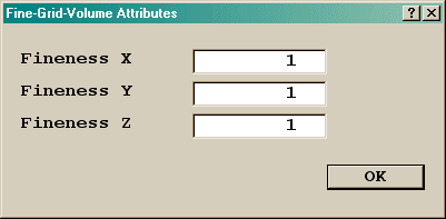
Image: OBJECT ATTRIBUTES
Fine grid volumes may be embedded within each other as deeply as required, with the constraint that each 'child' volume can only have one 'parent' - one volume cannot overlap two others, although they may touch at their boundaries.
Earth will disallow attempts to refine in directions in which the main grid has only one cell.
The default geometry for a fine grid volume is public\default\fine.dat.
Note that fine grid volumes are not compatible with:
A Transfer Object can either:
Images:
![]()
Default dialog
![]()
Export dialog
![]()
Import dialog
Transfer objects are part of the domain-partitioning technique, in which a large domain which is too large to model accurately on one computer is divided into a number of smaller domains, each of which can be handled by one computer. Each domain is solved in turn, starting with the most upwind ones. The technique is limited to cases where the flow is predominantly uni-directional.
At the end of each calculation, data describing the flow conditions on the downstream boundaries are placed into files which serve as 'transfer objects'; for the data can then be imported as upstream-boundary data for the later-to-be simulated next-downstream part.
As Transfer Objects are commonly placed at the same location as inlets and outlets, the Inlet and Outlet object types can also export and import the flow data thus removing the need for duplicate objects. A single Transfer Object can of course cover several inlets and outlets.
Current limitations are:
The assembly object has no attributes of its own. It acts as a 'container' for any number of other objects. Objects are added to an Assembly from the 'Hierarchy' button of the Object Dialog General page.
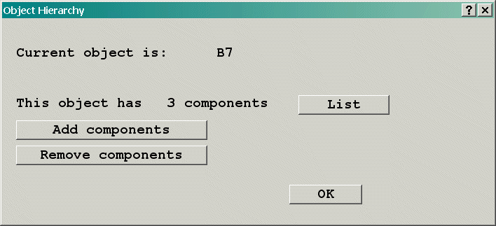
Image: Object Hierarchy Dialog
The 'Add components' button is the only one present for a new Assembly. It brings up a list of objects, from which the components can be selected. The 'List' button shows the names of the current components, and 'Remove components' removes selected objects from the component list.
Once an object has been made a component of an assembly, its individual 'Size' and 'Place' pages are disabled. The 'Size' and 'Place' pages for the assembly affect all the components of the assembly. The size and initial position of the assembly object should be set before any components are added.
To move a component of an assembly relative to the other components, select the component, and from the General page select Hierarchy. 'Disconnect' from the Assembly and close the Object dialog. The 'Size' and 'Place' pages will reappear the next time the Object dialog is opened. Make any changes required, then select Hierarchy again and 'Make into a component' to reattach to the Assembly object.
All the objects in an Assembly can be exported to a single file, for use in other models. This is done from the 'Export' button of the General page. The exported file, known as a POB (Phoenics Object) file, will be saved to the current working directory. To make it available in other projects using other working directories, copy it to a sub-directory of \phoenics\d_satell\d_object\users.
To import a saved Assembly, click on 'Object', 'New' 'Import Object'. Browse for the required POB file and select it. POBs can be imported from the local working directory, or from sub-directories of \phoenics\d_satell\d_object. All the component objects in the POB file will be imported. During the import process, a dialog will appear showing the position of the assembly, as read from the POB file. This can be changed as required at this stage, or the assembly can be moved later.
Note the following restrictions:
As mentioned above, the components of an assembly must have higher sequence numbers than the assembly object. If the assembly object is, for whatever reason, created after the components, the objects must be re-ordered before the components can be added to the assembly.
To do this, open the Object Management Dialog. Select the assembly object to be moved, and right-click in the 'reference' column. Using 'Line up' or 'Page up' or 'Top', move the object until it appears above all the component objects. Now proceed to add components to the assembly as normal.
Clipping plane objects can be created and manipulated in the Editor or Viewer.
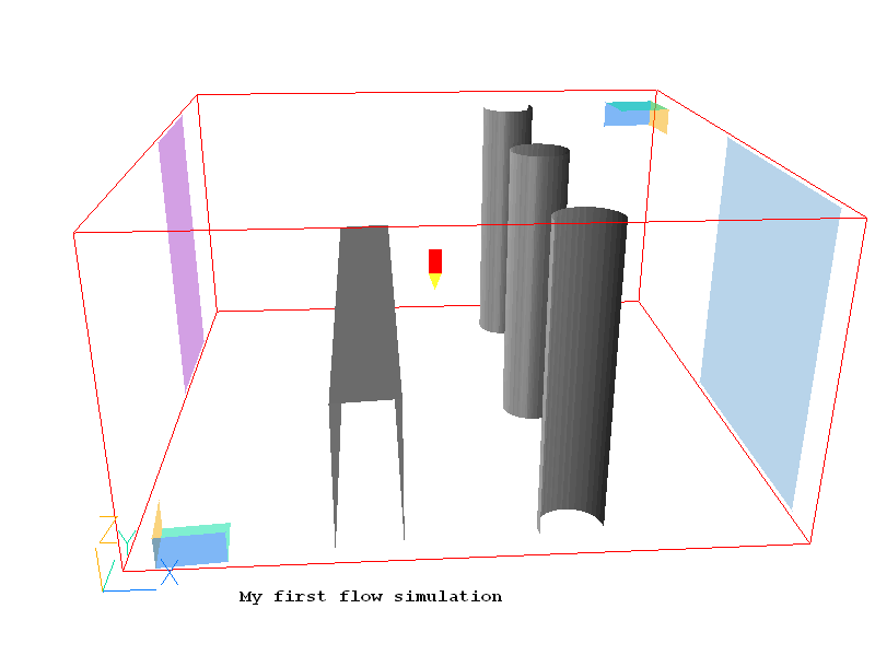
Each Clipping_plane object consists of 3 OpenGL clipping planes. A maximum of two such objects are allowed, as there are only 6 clipping planes. The first Clipping plane object is created at the origin, and clips everything 'behind' it. This is the left-hand object above. The second Clipping plane object is of type 'High end clipping plane' (on the Options tab), and is originally located at the far end of the domain This is the right-hand object above. It clips everything 'after' it. They can be moved and rotated at will to provide a better view inside objects or to remove (from view) items obscuring the area of interest.
Clipping plane objects can also be created from 'Settings - New - Clipping plane' on the Environment Settings menu, or 'Object - New - Clipping plane' on the Object Management Dialog. When created in the Editor, they will be written to the Q1 like all other objects whenever the Q1 is saved. When created in the Viewer, they will persist if the Editor is entered from the Viewer, but disappear if exit is to the system as Viewer never saves the Q1.
Clipping plane objects never affect the grid, and have no influence on the solution.
Plot surface objects can be created and manipulated in the Editor or Viewer, but their primary role is to aid visualisation in the Viewer.
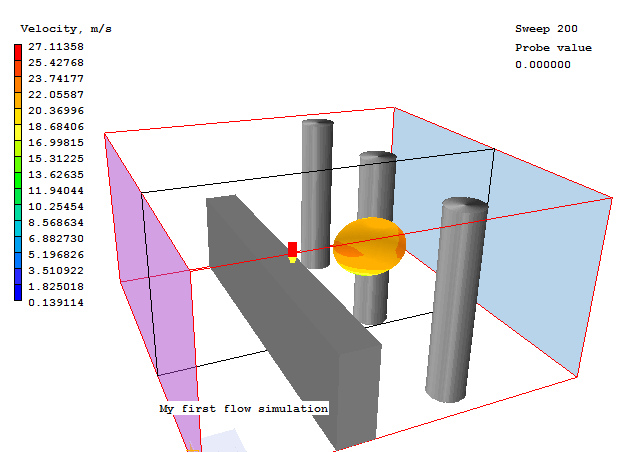
They can be any size and any shape. Once created, the Viewer can plot contours or vectors on the surfaces of the object.
Plot_surface objects can also be created from 'Settings - New - Plotting surface' on the Environment Settings menu, or 'Object - New - Plotting Surface' on the Object Management Dialog. When created in the Editor, they will be written to the Q1 like all other objects whenever the Q1 is saved. When created in the Viewer, they will persist if the Editor is entered from the Viewer, but disappear if exit is to the system as Viewer never saves the Q1.
Plot_surface objects never affect the grid, and have no influence on the solution.
Track_counter objects can be created and manipulated in the Editor or Viewer, but their primary role is to display and count VR-Viewer streamlines and / or GENTRA particle tracks passing through them. When selected, green dots mark where the track intersects the counter, and the red dots indicate the start points.
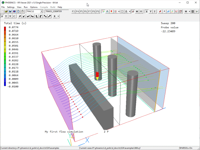
The track time for each track can also be displayed by:
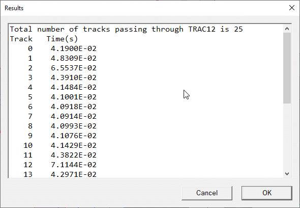
The data is automatically saved to a file named 'object_name.txt'.
If the case is transient, additional settings will appear on many of the above dialog boxes. A typical example is shown in the Inlet dialog box below:
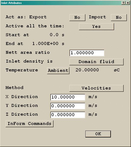
Image: ADDITIONAL SETTINGS
Active all the time Yes indicates that this inlet will be active for the entire duration of the transient. If Yes is toggled to No, the dialog box changes as shown below:
Image: INLET DIALOG BOX
The start and end times can now be entered. For the Earth run, the source will start in the time step which begins at, or closest to, the set start time and will end on the time step which ends at, or closest to, the set end time. Care should be taken to ensure that the time step settings will match the start and end times to a sufficient degree.
Note that the same time limits apply to all sources from a single object.
In a transient case, the following additional heat sources (marked by the vertical line) can be set, either for a blockage or a plate:
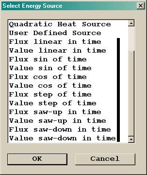
Image: ENERGY SOURCE
Typically, these extra time-varying sources require four additional settings. These are shown in the portion of the dialog box below, for Value step of time:
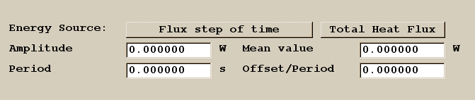
Image: VALUE STEP OF TIME
This will produce a heat source of the form:
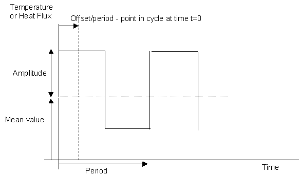
Image: TEMPERATURE OR HEAT FLUX
The extra settings have the following meanings:
When the time limits are set for an internal PLATE object, the porosity of the plate will also be affected. Before and after the set time period, the porosity will be set to 1.0. In other words, the plate only exists during the specified time period.
In a transient case, the name entered for either the export or import file is used as a base, and the time step number is appended before use. One file is written or read for each transfer object for each time step.
This is true whether the transfer is initiated from an Inlet, Outlet or Transfer Object.
Many objects types have a button labeled 'InForm Commands' on their attributes page. This leads to a dialog from which a selection of InForm commands can be attached to the current object. The usual format of an InForm command is as follows:
(KEYWORD of VARIABLE at LOCATION is FORMULA with CONDITION)
The dialog allows such commands to be created with the LOCATION keyword being taken as the name of the current object. InForm commands created in this way are held in the Q1 together with the remaining object attributes.
Image: INFORM SOURCES DIALOG - no settings
To create a new InForm command click 'Add InForm'. The dialog will now look like this:
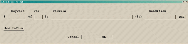
Image: INFORM SOURCES DIALOG - line added
The Keyword and Variable can now be selected from lists. To set the Keyword, click the button in the Keyword column:
Image: LIST OF KEYWORDS
The list of keywords is a sub-set of the full list of InForm commands. Their functions are
If one of the other InForm commands is needed, Go to the Main Menu, InForm Editor and use the traditional InForm format to set the command.
To set the variable, click the box under the 'Var' heading. A list of the variables currently STOREd or SOLVEd will be shown:
Image: LIST OF VARIABLES
Selecting 'New variable' displays a dialog on which the name of the new variable (up to 4 characters long) can be entered. If required, solution of the new variable can also be activated. New variables can also be created from the Main Menu, Models, Solution control / Extra variables panel.
The expression to be used as the 'formula' is entered by clicking on the button under the 'Formula' heading. An editing window will appear, in which the expression can be typed. The editor will be PQ1-Editor or Notepad, depending on the file editor selected under 'Options - Use PQ1Ed'.
Image: INFORM EDITOR
To save the expression and exit click 'File' then 'Save & exit'. In a similar way, any required condition for the expression can be entered into the 'Condition' column. Lines can be up to 1000 characters long. A $ can be freely used as the last character to act as a continuation-line symbol. When echoed to the Q1, the lines will be folded at column 68 regardless of how they were originally formatted. On the dialog, lines longer than the buttons will be shown as ending in '...'. The full expression will be shown in the editing window.
The 'Del' button will delete the current InForm line. As many InForm commands as required can be added to an object by repeatedly pressing 'Add InForm'.
As an example, the image below shows the settings required to make the inflow mass source and velocity at an INLET a linear function of the Z height.
Image: SETTINGS FOR MASS AND MOMENTUM SOURCES
Lines 1 and 2 set the mass source and momentum source to be linear with ZG, the Z height of the cell centre. The condition on line 1 states that the source is 'per unit area', and the condition on line 2 states that the mass source should be used as a multiplier (see the ONLYMS entry in the Encyclopaedia). Lines 3 and 4 create two local variables for InForm to hold the inlet velocity and density. Finally, lines 5 and 6 set the values for the inlet velocity and density.
When 'Use weather data file' is set to Yes, the WIND dialog changes to this:
IMAGE: WIND Dialog using weather data file
The next task is to select and then configure the data file by clicking Configure file.This leads to a dialog from which the file can be selected and read. The required data items can then be chosen.
When 'Use weather data file' is set to Yes, the SUN dialog changes to this:
IMAGE: WIND Dialog using weather data file
The next task is to select and then configure the data file by clicking Configure file.This leads to a dialog from which the file can be selected and read. The required data items can then be chosen.
IMAGE: Configure weather file
If weather data files in EPW format are already available, they can be selected by clicking NOTSET and browsing to the location of the file. If the required data file is not available, it can be downloaded from the EnergyPlus website by clicking on Start browser. This opens the EnergyPlus site on the page shown here:
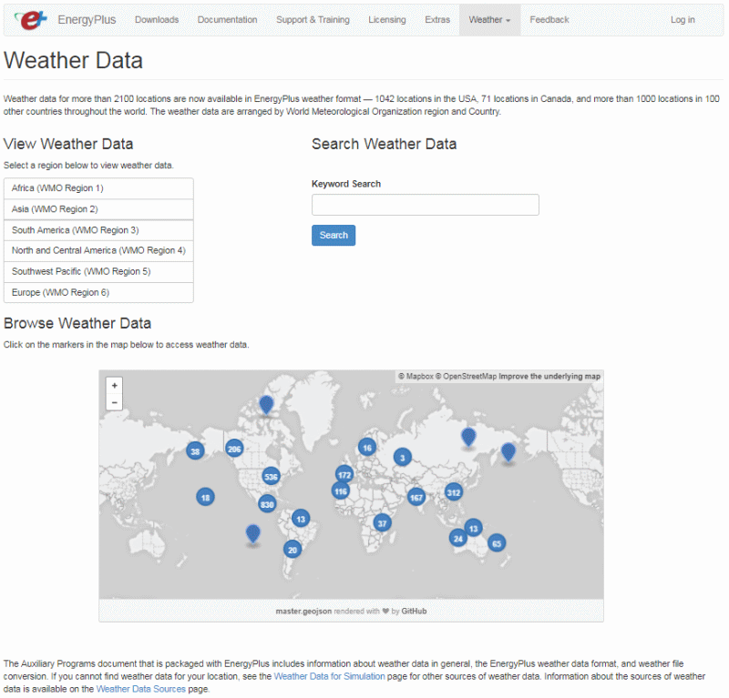
IMAGE: EnergyPlus web site
Choose a region, and then a country within that region. A list of available locations will be shown, for example from the United Kingdom:
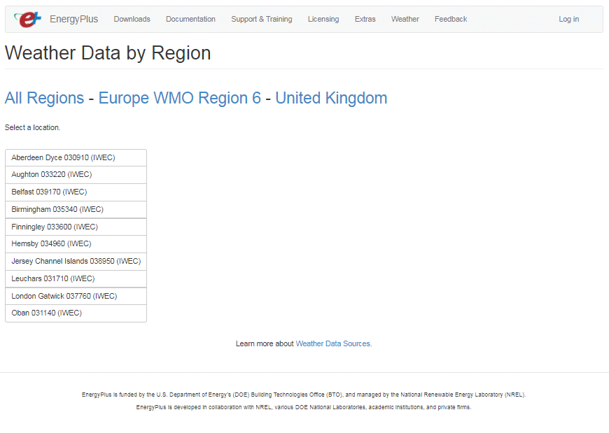
IMAGE: Select location on EnergyPlus web site
The ZIP file for each location contains a number of compressed files. Extract and download the one with the .epw extension, for example GBR_London.gatwick.037760_IWEC.epw. Save it to the current working directory, or any other convenient location. Once the file has been downloaded and saved, it can be attached. This is done by clicking NOTSET next to Weather data file and locating the file in the file browser that opens.
To change the weather file, follow the same procedure. When a weather file has been selected, the dialog shows the name:
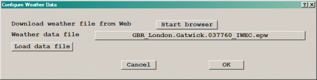
IMAGE: Weather data file selection confirmed
To read the data file, click Load data file. The dialog will update to show the WIND or SUN data that has been read.
The dialog will update to show what has been read:
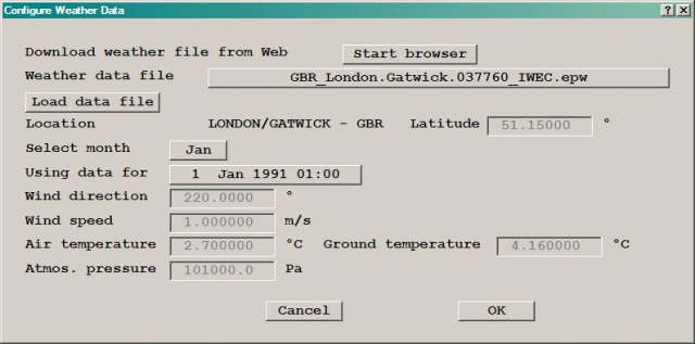
IMAGE: Weather data for WIND object
The data displayed are for the date and time shown. To select a different month, click the button next to Select month and select from the list. The data will change to that for the same day and time of the new month. To choose a different day and time, click the button next to Using data for, and scroll through the list of available days and times. The data is usually presented on an hourly basis for each day of the month. As shown in the example below, the selection dialog displays the wind direction, speed and air temperature for each entry in the file for the selected month.
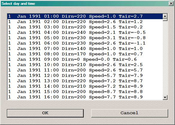
IMAGE: Example selection list for day and time - WIND
Once the date and time have been set, clicking OK on the Configure dialog will return to the Wind Attributes dialog. The data will update to reflect the chosen date and time.
The dialog will update to show what has been read:
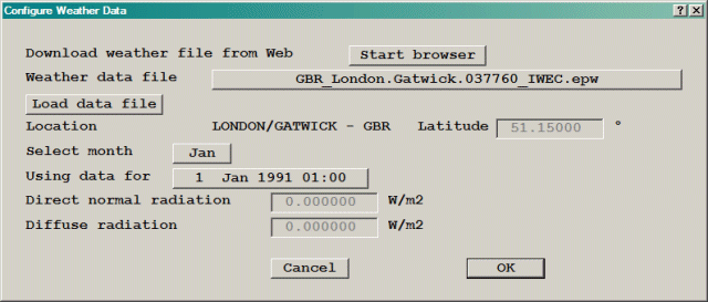
IMAGE: Weather data for SUN object
The data displayed are for the date and time shown. To select a different month, click the button next to Select month and select from the list. The data will change to that for the same day and time of the new month. To choose a different day and time, click the button next to Using data for, and scroll through the list of available days and times. The data is usually presented on an hourly basis for each day of the month. As shown in the example below, the selection dialog displays the direct and diffuse solar radiation for each entry in the file for the selected month.
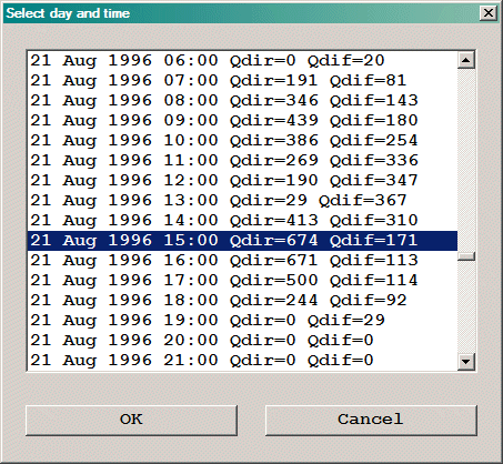
IMAGE: Example selection list for day and time - SUN
Once the date and time have been set, clicking OK on the Configure dialog will return to the SUN Attributes dialog. The data will update to reflect the chosen date and time.
The WIND_PROFILE object sets a single fixed-flow boundary using a logarithmic or power-law velocity profile. If the intention is to set conditions on all faces of the domain to represent wind flow, it is much easier to use the WIND object, described above.
IMAGE: WIND_PROFILE dialog
The inlet boundary conditions associated with a wind velocity profile (the atmospheric boundary layer) can be specified by using a WIND_PROFILE object. Either a logarithmic or power-law velocity profile can be specified, as follows:
U/U* = ln((z-d)/zo )/ κ
U/Ur= (z/zr)α
and the turbulence quantities are set to:
k = U*2/√(CμCd); ε= U*3/(κ*z)
or, for the k-omega model:
k = U*2/√(CμCd); ω= U*/(κ√(CμCd)z)
where U is the total velocity at the height z from the ground; κ is von Karman's constant (=0.41), zo is the effective roughness height of the ground terrain; Ur is the reference velocity at the reference height zr, and α is the power-law exponent. The total friction velocity U* is given by:
U*= Ur κ/ln((zr-d)/zo)
Typical values of the roughness height zo and the power-law exponent a are given in the table below:
| Surface type | Roughness height zo (m) | Power-law exponent α |
| Open flat terrain, grass, few isolated obstacles | 0.03 | 0.13 |
| Open sea | 0.0002 | 0.16 |
| Low crops, occasional large obstacles | 0.10 | 0.16 |
| High crops, scattered obstacles | 0.25 | 0.19 |
| Parkland, bushes, numerous obstacles | 0.50 | 0.21 |
| Suburb, forest, regular large obstacle coverage | 0.50 to 1.0 | 0.21 to 0.24 |
The roughness height should not be greater than the height of the first cell-centre above the ground as this may lead to numerical problems.
The reference height zr is usually taken as 10m because this is the height at which mean wind data are generally provided.
The zero-plane displacement d is the height above the ground at which zero wind speed is achieved as a result of flow obstacles such as trees or buildings, ie Ur=0.0 at z=z0+d. Often the displacement height is zero, but for flow over an array of densely packed objects (e.g. a forest, cropland or buildings), an offset in height is introduced into the log law to allow for the upward displacement of the flow by the surface objects. This displacement height d is usually estimated as 2/3 of the average height of the obstacles.
The displacement height d is a positive quantity, although the user can set d=-z0 to use wall functions that are consistent with the inlet wind profiles proposed by Richards & Hoxey (1993)11, which are often used in wind-engineering simulations.
Engineers often prefer to use a power law profile, although the log law is to be preferred because it is based on physical laws rather than on an empirical formulation. A commonly-used empirical relationship between α and z0 is:
α = 0.096 log10 (zo) + 0.016 [log10 (zo)]2 + 0.24
The height above the ground, z, is measured from the first open cell in each column of cells. This allows the profile to follow the terrain imposed by a blockage.
IMAGE: Wind profile starting over a terrain
A density is required to calculate the mass flow rate. If the 'Inlet density is' is set to Domain fluid, the density will be taken from the formula selected for the domain fluid in the Main Menu, Properties panel. The density will be calculated from the values set at the boundary location.
If the fluid entering is not the domain fluid, the setting can be switched to User-set. In this case, the required inlet density can be set directly. (This is the default for complex density relationships).
Inlet values for solved scalars are set by selecting the scalar with the Setting scalar button, then specifying the required inlet value.
Radiative Heat Loss
If the IMMERSOL radiation model is active, the wind profile boundary can be allowed to exchange heat by radiation with the surroundings. If the External radiative link is set to Yes, the temperature of the surroundings, Texternal, can be set. The heat flux from the wind profile boundary will then be:
Q" = σ (Text4 - Tp4) (W/m2)
Internal Wind profiles
If the wind profile boundary is internal to the domain, an extra button appears on the dialog box, labeled Object side. The settings for this are Low or High, and they indicate whether the inflow is to appear on the low-co-ordinate face or high-co-ordinate face of the object. The flow direction determines whether the boundary acts as a source or sink.
GENTRA Particle Tracker
If the Lagrangian Particle tracker GENTRA is active, the wind profile boundary will act as a particle exit by default. This can be switched off.
Restrictions
The following restrictions apply to the wind_profile object:
InForm Commands
This leads to a dialog from which a selection of InForm commands can be attached to this object. It is described in InForm Commands below.
This is like the User Defined object, except that instead of forcing the grid to match the faces of the object, any related source is applied to the cells whose centres happen fall within the object. It is frequently used to define a fixed-pressure cell in a closed volume. The default geometry is public\default\box.dat and the default colour is khaki (colour 56), representing a khaki cuboid.
A User_defined object set to not affect the grid is exactly equivalent to a Celltype object.
The PCB (Printed Circuit Board) object behaves as a Blockage, with the exception that:
The default geometry for a PCB is public\default\box.dat and the default colour is green (colour 121), representing a green cuboid.
The Drag_lift object has no attributes. It defines a volume over which a momentum balance will be performed. The pressure, convection and diffusion fluxes are summed over the six faces of the bounding box of the object. The resulting force is printed to the RESULT file if 'Output of forces and moments' has been set to 'On' in the Main Menu - Output panel.
1. Finnigan, J., "Turbulence in plant canopies", Annual Review of Fluid Mechanics, 32:519-571, (2000).
2.Svensson, U. & Haggkvist, K., "A two-equation turbulence model for canopy flows", Journal of Wind Engineering and Industrial Aerodynamics, 35:201-211, (1990).
3.Green, R.S., "Modelling turbulent air flow in a stand of widely-spaced trees", PHOENICS Journal, 5:294-312, (1992).
4.Liu, J., Chen, J.M., Black, T.A. & Novak, M.D., "k-ε modelling of turbulent air flow downwind of a model forest edge". Boundary-Layer Meteorology, 72:21-44, (1998).
5.Sanz, C. "A note on k-ε modelling on a vegetation canopy", Boundary-Layer Meteorology", 108:191-197, (2003).
6.Krzikalla, F., "Numerical investigation of the interaction between wind and forest under heterogenous conditions", PhD Thesis, Institute for Hydromechanics, University of Karlsruhe, (2005).
7.Lopes da Costa, J. C. "Atmospheric Flow over Forested and Non-forested Complex Terrain", PhD thesis, University of Porto, (2007).
8. Huang, J., Cassiani, M. & Albertson, J., "The effects of vegetation density on turbulent structures within canopy sublayer", AMS, Paper 2.2, (2008).
9.Zeng, P. & Takahashi, H., " A first-order closure model for the wind flow within and above vegetation canopies", Agricultural and Forest Meteorology 103: 301-313, (2000).
10.Van Renterghem, T. & Botteldooren, D., "Numerical evaluation of tree canopy shape near noise barriers to improve downwind shielding", J.Acous. Soc. Am., 123(2), 648-657, (2008).
11. Richards,P.J. & Hoxey,R.P., "Appropriate boundary conditions for computational wind engineering models using the k-ε turbulence model." J.Wind Engng & Industrial Aerodynamics, 47, 145-153, [1993] ).
12. Zhang,M., et al, “The Effects of the Layouts of Vegetation and Wind Flow in an Apartment Housing Complex to Mitigate Outdoor Microclimate Air Temperature”, Sustainability 11(11), 3081 (2019).
13. Mo, J.B.; Wang, L.M.; Qin, J.; Huang, J.; Hu, Y.H.; “Study on temperature decreasing and humidification of ornamental plants in Shanghai.”, J. Anhui Agric. Sci. (2007), 35, 9506–9507. (In Chinese).