
This section describes the menus and dialog boxes available from the top bar of the main VR-Editor/Viewer graphics window. In some cases, the same functions can be accessed via the icons on the tool bar.
File Menu, Settings Menu, View Menu, Run Menu, Multi-Run Menu, Options Menu, Compile Menu, Build Menu, Help, The Tool Bar, The Status Bar
The File menu consists of the following items:
Start new case, Open existing case, Load from libraries, Reload Working files, Open file for editing, View monitor plot, Save working files, Save as a case, Save Q1 File As, Copy Window to Clipboard, Save Window As, Print, Exit, Quit
This will bring up a list of available Special-Purpose Products (SPPs).
 .
.
Core is the general-purpose menu, which is normally supplied to users; the others are Special-Purpose Programs that are supplied only as a result of a specific order.
Selecting one of them wipes out all the settings for the current case, and resets all variables to their default values. All the default input and output files (see File - Save as a case) are deleted. If intermediate solution files are present, the grayed-out items in the 'Delete intermediate step files' box become active, asking whether they should be deleted as well.
A new Q1 is created, which contains the following lines:
TALK=T;RUN(1,1)
CPVNAM=VDI; SPPNAM = sppnam
STOP
where sppnam is the name of the selected Special-Purpose Program.
This function is also accessed from the ![]() icon on the toolbar.
icon on the toolbar.
If 'Preserve current view location' is ticked prior to clicking 'OK', the view information held in the new case will be ignored, and the current view will be preserved. This can be useful when comparing details of different cases.
This allows a
previously saved case to be read in (see File - Save as a
case). This function is also accessed from the ![]() icon on the
toolbar.
icon on the
toolbar.
A dialog box is opened requesting the user to confirm that an existing case is to be opened. Before the dialog is opened, a check is made to see if intermediate step or sweep files are present (see Main Menu - Output, Field Dumping for information on how to save intermediate files). If they are present, the dialog will also ask whether to delete the intermediate files.
If 'Open case in current directory' is selected, the current working directory is left unchanged, and files will be copied into it.
If 'Open case in case directory' is selected, the working directory will be changed to the folder where the case files are stored. This will allow any geometry files specific to the case to be picked up.
The current working directory is the one in which the program started, unless it has been changed since. The working directory can be changed from ' Options - Change working directory'.
If the VR-Environment was started from the command line, it is initially whatever directory the command was issued from.
If it was started from the Start menu, or by clicking on the PHOENICS icon, it is the last working directory used the previous time PHOENICS was run. By default, it is set under 'Properties / Start in' for the Start menu item or icon to \phoenics\d_priv1.
If 'Preserve current view location' is ticked prior to clicking 'OK', the view information held in the new case will be ignored, and the current view will be preserved. This can be useful when comparing details of different cases.
If 'Delete solution output files' is ticked prior to clicking 'OK', then the set of solution files in the working directory will be deleted. This will force the Viewer to search for solution files in the case directory.
If 'Delete Graphical monitoring files' is ticked prior to clicking OK, any intermediate monitoring files in the working directory will be deleted.
If 'Delete Particle tracking files' is ticked prior to clicking OK, any intermediate GENTRA track files in the working directory will be deleted.
When 'Select Case' (or 'OK') is clicked, a further dialog opens, which allows browsing for files with a .Q1 extension.
The files for the selected case are then copied to the selected working directory under their default names - see File - Save as a case for a list of default names.
This function may be accessed from the Open case icon
 on the toolbar.
A saved case may also be opened by dropping it into the VR-Editor window. To do this, highlight a Q1 file in an opened Windows Explorer window, and then, with the left mouse button held down, drag it into the VR-Editor (or VR-Viewer) window and release the mouse.
Once a case has been opened, the case name is displayed in the status bar at the bottom of the VR-Editor window.
The dialog box below allows a case to be loaded from one of the PHOENICS libraries.
If the case number is known, it can be entered directly into the case-number entry box. To browse through the libraries to find a suitable case, click on Browse. This brings up a library-browsing dialog:
The various trees can be expanded by clicking on the + next to the library name.
This causes VR-Editor to read the data in the Q1 file on disk in the current working directory. This has the effect of removing all changes made since the last time the working files were saved, or the case was saved.
Any changes made to the Q1 file by hand editing will be acted upon.
This opens one of the following files for editing with the selected text editor (by default PQ1ED, though this can be changed to Notepad from the Options menu.):
'New' Convergence Monitor
This opens a window which displays the latest convergence monitor plots generated by the Earth solver.
The plots are:
'Classic' Convergence Monitor
This opens a window which displays the latest convergence monitor plots generated by the Earth solver.
The plots are:
according to the settings made in the Q1. These setting can be made using the Monitor options dialog from the Options menu.
If the "Save all 4 monitor views at the end of run" option is ticked on that dialog, then the menu option for each of the plot types is enabled here.
This causes VR-Editor to write out a Q1 file to the current working directory, based on the current settings. The existing Q1 will be overwritten. EARDAT and FACETDAT files for Earth are also written if asked for.
This will save the Q1 input file and all relevant output files by copying them as detailed in the table below. Firstly a dialog asks if changes to the Q1 are to be saved.
By default, the Q1 file on disk will be used if there is already a RESULT file present, and the RESULT file is newer than Q1. This implies that an Earth run has already been made. In that case, the Q1 on disk is likely to be the one used for the solution. If there is no RESULT file present, the default is to overwrite the Q1 on disk with the current setup before saving the file.
If 'Save changes' is ticked, the Q1 on disk will be overwritten with the current setup. If it is not, the Q1 on disk will be used. It is not necessary to save changes to EARDAT at this point. After clicking 'OK', a file-browsing window will open, as shown below,
Select a folder, or make a new one with the new folder icon. Enter a name into the File name box and click Save. The default folder is the current working directory. Save to a different folder by browsing to it or making it in the file selector.
The following files are saved ('case' represents the file name entered in the 'Save As' dialog):
| File name | Function | Saved as: |
| q1 | Input file | case.q1 |
| result | Results file | case.res |
| phi1 | ASCII solution-field file | case.phi |
| phida1 | direct-access solution-field file | case.pda |
| parphi | ASCII solution-field file for PARABOLIC or 2D-XY transient | case.par |
| parada | direct-access solution-field file for PARABOLIC or 2D-XY transient | case.pdr |
| pbcl.dat2 | PARSOL cut-cell data file | case.pbc |
| xyz3 | ASCII BFC grid file | case.xyz |
| xyzda3 | direct-access BFC grid file | case.xda |
| patgeo | PHOTON geometry file | case.pat |
| gxmoni.gif | EARTH monitoring image from last solution sweep (Classic monitor) | case.gif |
| gxmoni_spot.gif | EARTH spot-value image from last solution sweep (Classic monitor) | case.spot.gif |
| gxmoni_mxcr.gif | EARTH maximum correction and residual image from last solution sweep (Classic monitor) | case.mxcr.gif |
| gxmoni_mnmx.gif | EARTH maximum/minimum value image from last solution sweep (Classic monitor) | case.mnmx.gif |
| gxmoni_mxc.gif | EARTH maximum correction image from last solution sweep (Classic monitor) | case.mxc.gif |
| convergence-spot.png | EARTH spot value image from last solution sweep (New monitor) | case.convergence-spot.png |
| convergence-residual.png | EARTH residual value image from last solution sweep (New monitor) | case.convergence-residual.png |
| convergence-maxcorrection.png | EARTH maximum correction value image from last solution sweep (New monitor) | case.convergence-maxcorrection.png |
| convergence-netsource.png | EARTH nett source value image from last solution sweep (New monitor) | case.convergence-netsource.png |
| convergence-domainmin.png | EARTH domain minimum value image from last solution sweep (New monitor) | case.convergence-domainmin.png |
| convergence-domainmax.png | EARTH domain maximum value image from last solution sweep (New monitor) | case.convergence-domainmax.png |
| ghis4 | file containing GENTRA particle track histories | case.his |
| gphi4 | GENTRA restart file | case.gphi |
| genuse4 | macro file for drawing GENTRA particle tracks | case.gen |
| u | PHOTON 'USE' (macro) file | case.u |
| inforout | output file from In-Form PRINT | case.inf |
| cham.ini | configuration file | case.init |
| phoenics.mcr | Tecplot macro file | case.phoenics.mcr |
| tecgeom.dat | Tecplot geometry file | case.tecgeom.dat |
| tecdata.dat | Tecplot formatted solution file (32-bit) | case.tecdata.dat |
| tecdata.plt | Tecplot unformatted solution file (64-bit) | case.tecdata.plt |
| fvgeom.fvuns | Fieldview geometry file | case.fvgeom.fvuns |
| fvformula.frm | Fieldview macro file | case.fvformula.frm |
| fvdata.nam | Fieldview name file | case.fvdata.nam |
| fvdata.g | Fieldview grid file | case.fvdata.g |
| fvdata.f | Fieldview solution file | case.fvdata.f |
| phi.vtk | VTK solution file | case.phi.vtk |
| uspphi | Unstructured PHOENICS solution file | case.uspfi |
| obj_faces.vtk | Unstructured PHOENICS object faces file | case.obj_faces.vtk |
| conv_table.csv | Convergence table (Flair only) | case.conv_table.csv |
| heat_sources.csv | Fire object heat source table (Flair only) | case.heat_sources.csv |
| smoke_sources.csv | Fire object smoke source table (Flair only) | case.smoke_sources.csv |
| fandata | Fan flow characteristic file (Flair only) | case.fan |
| rad.dat | Radiation view-factor output file (CVD only) | case.rad |
| radi.dat | Radiation view-factor input file (CVD only) | case.radi |
| minires.htm | Reduced convergence infoprmation report | case.minires.htm |
| pardat | Parallel-PHOENICS manual domain splitting file | case.pardat |
Notes:
The files will be copied to the selected folder. Warnings are issued if files with the
same name already exist, or if the Q1 is newer than RESULT. This function is also accessed
from the ![]() icon on the tool bar.
icon on the tool bar.
Once the above files have been saved, a check is made to see if intermediate step or sweep files are present (see Main Menu - Output, Field Dumping for information on how to save intermediate files).
If they are present, a second dialog opens, asking whether these should be saved as well. If it is chosen to save them, a new folder will be created named <case_name>, and they will be moved into this new folder. e.g. for case run_1 saved to folder case_1, the folder run_1 will be created in case_1, and the names would be case_1\run_1\a1, case_1\run_1\a2 etc.
If PARSOL is active, the intermediate cut-cell data files will be saved as <case_name>.pbc<letter><number> e.g. case_1\run_1\pbca1, case_1\run_1\pbca2 etc.
If GENTRA is active, intermediate GENTRA restart files will be saved as <case_name>. gphi<letter><number>.
Once a case has been saved, the current case name is echoed in the status bar at the bottom of the VRE screen.
This will save the Q1 as a new file with a different name. Firstly a dialog asks if changes to the Q1 are to be saved.
If 'Save changes' is ticked, the Q1 on disk will be overwritten with the current setup. This is the default. If it is not, the Q1 on disk will be used. After clicking 'OK', a file-browsing window will open. Select or make a folder, enter a name and click 'Save'. The Q1 on disk will be copied to the new name.
The window contents are saved to the clipboard for pasting into another program.
This allows the contents of the main graphics window to be saved as a GIF, PNG, BMP or JPG format file.
The dialog box allows the pixel size and aspect ratio for the saved image to be selected. The default resolution and aspect ratio are the same as those of the original screen image. The Reset button sets the height and width to the current height and width of the graphics window.
The default file type is set in the [Graphics] section of the CHAM.INI file.
This function is also accessed from the ![]() icon on the tool
bar.
icon on the tool
bar.
Note that if 'Use virtual screen' is ticked, the area of the main graphics window is captured without any overlying windows and without the surrounding window frame and toolbars. If the hand-set is moved to lie over the main graphics window, it will not be included in the saved image.
If 'Use virtual screen' is unticked, the entire window together with frame, toolbars and any overlapping windows will be captured.
The image will be saved with whatever background colour has been set from ' Options - Background colour'.
The default folder is the current working directory.
Users wishing to save in PCX format should add '.pcx' to the file name entered, and a pcx of that name will be saved.
This allows the contents of the main graphics window to be sent directly to any available printer device.
The dialog box allows the printer, number of copies and other print options to be
selected. This function is also accessed from the ![]() icon on the tool
bar.
icon on the tool
bar.
The image will be saved with whatever background colour has been set from ' Options - Background colour'.
This exits from PHOENICS. Before the program closes down, a prompt to save the current work will be given .
This exits from PHOENICS without saving any files. PHOENICS-VR can also be exited without saving by clicking on the Close window icon, in the top-right corner of the main graphics screen.
The Settings menu consists of the following items:
Domain Attributes, Probe Location, Add Text, New, Object Attributes, Find Object, Datmaker Operations, Editor Parameters, Graphics Options, View Direction, Near Plane, Rotation speed, Zoom speed, Depth effect
This
brings up the Main Menu. It is
equivalent to the 'Main Menu' button  on the hand-set,
the
on the hand-set,
the  icon on the toolbar,
or double-clicking the DOMAIN object in the
Object Management Dialog.
icon on the toolbar,
or double-clicking the DOMAIN object in the
Object Management Dialog.
In the
Editor, the probe location defines the location in the model domain which will be used to
monitor the progress of the solver solution. It is represented visually in the domain as  . The probe
location dialog allows the user to locate the probe either using physical units within the
domain or via cell location.
. The probe
location dialog allows the user to locate the probe either using physical units within the
domain or via cell location.
Set view centre will set the view centre of the image to the current probe location, thus centering the image on the probe.
Appearance toggles the display of the probe between the default 'pencil', and an alternative sphere. When a sphere is chosen, the third button in the row opens a colour-chooser to set the colour of the sphere. The colour of the 'pencil' probe cannot be changed. The data-entry box under the buttons (showing 1.000000 in the image) controls the relative size of the probe.
The 'Parameters' tab is described under 'Settings - Editor Parameters'.
This option can be used to place up to twenty lines of text on to the main graphics window. To create a new text object, select 'Add' from the Text menu. This will open the Text Properties dialog (shown below).
Each line of text may be up to 80 characters in length. The text may be placed in the window either by specifying a pixel location or by clicking the left mouse button over the desired location.
The 'Attributes' menu may be used to change some of the attributes of the text, e.g. colour. The font used for the text will be that specified by the 'Choose Font' item on the Options menu.
Note: The text is not saved to Q1, so is lost on exiting the VR Environment. In the Viewer, text items are saved to a macro.
 .
.
There are six options -
New Object displays a list of all object types currently available. This will depend on the chosen Special Purpose product. The object types supported by Core PHOENICS are given in Object Types and Attributes.
Selecting one creates a new object of that type and displays the object dialog for the newly-created
object. It is equivalent to clicking on Object - New - New Object in the Object management
Dialog reached from 'Object' button  on the hand-set
or the
on the hand-set
or the  icon on the toolbar.
Import CAD Object
Creates a new object and opens the CAD Import dialog for it.
Import CAD Group
Opens the Group CAD import dialog, which allows a number of CAD files to be imported in one action. Each CAD file specified will create a new object.
Import Object displays a file-browser, with which a pre-existing assembly (POB) file can be selected for import. New objects are generated for each object in the assembly, and the object dialog for the first object in the assembly is displayed.
Clipping plane creates a new Clipping_plane object.
Plotting Surface creates a new Plot_surface object.
Track_counter creates a new Track_counter object.
This brings up the object dialog box for the currently-selected object. It is equivalent to double-clicking on an object. If no object is already selected, the Object Management Dialog, showing a list of all objects, will be displayed.
This brings up the Object Management Dialog. The selected object (if any) becomes the current object, and is high-lighted in the list of objects.
This brings up the Datmaker Operations dialog, which allows various operations to be carried out on one or more objects.
If no object is pre-selected, then the domain "CHAM" will be displayed in the first line and the listbox will be empty. The first object may be selected either by clicking on an object in the domain or by selecting one from the pulldown list.
For a single object, the following repair operations are available:
Note that the more repair processing is selected, the longer the repair may take.
Once a first object has been selected and 'Object changes' is ticked, then a list of compatible objects will appear in the 'Other objects' listbox - for an object to be considered compatible it must be of the same Object Type (eg BLOCKAGE) and have the same Material Property as the first. Several objects can be selected using standard Windows selection techniques.
The following operations can then be performed:
After a Union or Merge operation a new object is created with size and position set to just encompass all the merged objects. The original objects are all reset to NULL, and the new object is set to not affect the grid in order to keep the mesh the same.
The user can provide a filename for the modified object geometry, the initial default being 'mygeom.dat', but if this already exists then the name will increment to 'mygeom_1.dat' etc.
The default is to save any changes to the q1 before carrying out the selected operations. This Q1 is copied to another name, the initial default name being 'saved.q1', but if this already exists then the name will increment to 'saved_1.q1' etc. This enables the user to revert to the pre-operations Q1 if necessary.
The VR Editor Parameters menu sets the Increment size and Scale factors.
- Increment controls the increment in size or position each time the Size up/down or Position up/down buttons on the hand-set are pressed. It also controls the incremental movement of the probe. There is a separate increment size in each coordinate direction, defaulted to give approximately 100 steps to cross the domain. This can be useful if the domain dimensions are very different in each direction.
- Snap to grid, when ticked, forces the size and position of objects and the probe position to be exact multiples of the increment size when the up/down arrows are clicked. When not ticked (the default), the size and position will change by the increment from the current size/position. Note that this function applies to the Size and Place tabs of the Object dialog, not the hand-set. Exact values can always be typed in.
- The scale factors control the relative scaling of the entire geometry. If the aspect ratio of the domain is extreme, say the domain is 100m * 1m *100m, it is very difficult to visualise the domain properly. It can also be difficult to select objects, as one of their dimensions will be very small. In such a situation, setting the scale factors to 1, 20, 1 would make the domain appear to be 100 * 20 * 100
The Probe tab is described under 'Settings - Probe location'.
This dialog controls which rendering options are used and how the scene is illuminated. It can also be reached
by a left-click on the Graphics Options icon  on the toolbar. A right-click on this icon toggles the VBO shadows on and off.
The first item selects the rendering engine to be used:
When 'with shadow' is ticked, the objects in the domain will cast shadows. The shadows are cast by the default lighting as set by the 'Light source location' further down the dialog. This is the default rendering option.
If a SUN object is present, then the shadows are cast by the sun.
When 'with shadow' is not ticked, the display of shadows is turned off. This also applies to shadows cast by the SUN object. This function can be toggled by right-clicking the Graphics Options icon
on the toolbar.
For the 'Simple Shader' an additional button appears:
This allows a base colour for the simple shading to be selected. The 'simple' colours are chosen by swapping the red and blue components of the chosen colour to make the contrast colour.
Light effect (VBO only) The intensity controls the amount of lighting effect applied to all objects regardless of the light source position. A light effect of zero means that areas unlit by the diffuse light source receive no lighting at all and are entirely black, while areas lit by the diffuse light source get only the effect of that light. Larger values produce more lighting effect in areas not lit by the diffuse light source, making these areas show some of the surface color. An ambient light of 100 means that all areas are lit by the maximum amount, and areas unlit by the diffuse light source use the full surface color. With zero light, shadows cannot be displayed.
Material specularity (VBO only) Specular Highlighting adds the semblance of reflected light to 3D shaded or flooded objects. The intensity (%) controls intensity of specular highlights (that is, the amount of reflected light, which controls the amount of whiteness at the peak of the highlight).
Light ambient: (Legacy shader only) Turns the ambient light on and off. The intensity controls the amount of lighting effect applied to all objects regardless of the light source position. An ambient light of zero means that areas unlit by the diffuse light source receive no lighting at all and are entirely black, while areas lit by the diffuse light source get only the effect of that light. Larger values produce more lighting effect in areas not lit by the diffuse light source, making these areas show some of the surface color. An ambient light of 100 means that all areas are lit by the maximum amount, and areas unlit by the diffuse light source use the full surface color.
Light diffuse: (Legacy shader only) Turns the directional light on and off. The intensity controls the amount of lighting effect produced by this light source. An intensity of 100 produces the maximum contrast between lit and unlit areas, and fully lit areas use the full surface color. Lesser values produce less contrast between lit and unlit areas, and fully lit areas use darker colors. An intensity of zero means the light source produces no contrast between lit and unlit areas, and all areas are black.
Light specular: (Legacy shader only) Turns specular highlights on and off for all light-source shaded objects in the plot. Specular Highlighting adds the semblance of reflected light to 3D shaded or flooded objects. The intensity (%) controls intensity of specular highlights (that is, the amount of reflected light, which controls the amount of whiteness at the peak of the highlight).
Light source location: (All shaders) The light source is attached to the domain, so the lighting does not change as the domain is rotated. The upper slider moves the light through 360 in the X-Y plane, and the lower slider through 360 in the Y-Z plane. When both sliders are at zero (at the left end), the light shines straight down the Y axis.
Secondary opposing light source: (Legacy shader only)Turns on and off a second light source directly opposite to the main light source. This lights the back of the model, giving a fairly uniform illumination.
This option leads to the Reset View Parameters dialog which is described in the section Reset View Parameters.
Parts of the image closer than the near plane are not visible. The default setting ensures that the entire image is visible. The near plane can be moved interactively by sliding the slider on the dialog box. The dialog can remain open without interrupting other activities. Reset restores the default value.
Image:INCREASED NEAR PLANE
Rotating and zooming the image will expose or hide different parts of the geometry. The introduction of 3D clipping plane objects has reduced the need of using the near plane for exposing parts of the geometry.
Note that the backs of the exposed facets are transparent. This is because in a valid solid model all facets point outwards. To draw all facets double-sided to appear solid, click on View, Show back of objects. If switching the display of backs of objects leads to unexpected changes in the image, it is likely that the geometry file is faulty and has some facets pointing in not out. This can often be repaired by Datmaker.
Image:INCREASED NEAR PLANE (with visible backs)
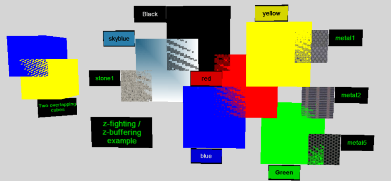
Note that setting the Near Plane to too small a value can lead to a phenomenon known as Z Fighting where two coplanar polygons cannot be drawn cleanly, as shown in this example from Wikipedia:
Rotation speed controls the speed at which the image rotates in response to the 'rotate' and 'move' buttons on the hand-set or mouse movements.
The rotation speed can be changed interactively by sliding the slider on the dialog. The dialog can remain open without interrupting other activities. Reset restores the default value.
Zoom speed controls the rate at which the image gets bigger or smaller in response to the hand-set 'zoom' buttons or mouse movements.

The zoom speed can be changed interactively by sliding the slider on the dialog. The dialog can remain open without interrupting other activities. Reset restores the default value.
Depth effect controls the degree of perspective visible. Another way of controlling this is the Angle Up/Angle Down button-pair.
Image: Large depth
effect
Image: Small depth effect
The depth effect can be changed interactively by sliding the slider on the dialog. The dialog can remain open without interrupting other activities. Reset restores the default value.
The View menu contains the following items:
Control Panel, Movement control, Toolbars, Status bar, Text box, Show back of objects, Window size
This controls whether the object and domain hand-set is visible or nor. The hand-set can be closed by clicking on the 'close window' icon in the top-right corner. This may be required, for example, in order to get an unobstructed full-screen image. Once closed, the hand-set can only be restored from this menu. When the hand-set is closed, additional buttons appear on the toolbar in order to maintain functionality.
This controls whether the movement hand-set is visible or nor. The hand-set can be closed by clicking on the 'close window' icon in the top-right corner. This may be required, for example, in order to get an unobstructed full-screen image. Once closed, the hand-set can only be restored from this menu.
When the movement hand-set is closed, the mouse control is automatically activated.
This controls which parts of the toolbar appear at the top of the graphics screen. The toolbar can be used to replace the functions of either hand-set.
The 'general' toolbar contains the file-handling icons, and also displays the name and type of the currently selected object. If no object is selected, it will display the name of the domain, usually set to CHAM.
![]()
The 'domain' toolbar contains icons connected to the domain, including the probe and Main Menu.

The 'Object' toolbar contains icons connected with object management.
![]()
The 'Movement' toolbar contains the movement icons from the Movement handset.
![]()
'All' displays all the currently available portions of the toolbar.
The tool bar is automatically turned off if the BFC mesh generation menu is entered.
This controls whether the status bar along the bottom of the graphics image is visible or not.
This controls whether the Satellite command prompt should be visible or not. If a Q1 being loaded into the VR-Editor requires a response from the user, or if errors are detected reading the Q1 file the Command prompt will be automatically made visible regardless of this setting.
By default, the facets defining the objects are only drawn single-sided. If holes appear, it is likely that some facets are pointing the wrong way, and the object is not valid. If the 'Near Plane' setting or a Clipping Plane object has been used to cut away part of the geometry, then again the transparent backs of some facets will be exposed. To make them appear solid, toggle the tick-mark next to Show backs of objects.
This causes the current window size to be displayed at the right-hand end of the Status bar at the bottom of the screen.
The Run menu consists of the following items:
Pre processor, Parallel Solver, Solver, Post processor, Utilities
The Pre processor sub-menu contains the following items:
GUI - Pre processor (VR Editor),Text mode (Satellite), Fortran creator (Plant Menu), CHEMKIN Interpreter
This option is grayed out when the VR-Editor is active. In the VR-Viewer, it is the way to switch to the VR-Editor.
This will run the PHOENICS Satellite, using the Q1 file in the current working directory.
The PLANT menu is a graphical environment for the creation of Fortran code, which is linked into the Earth Solver. Expressions are provided, in algebraic form, for physical properties, source terms, specialised output. PLANT turns these expressions into error-free Fortran. For a description of PLANT, click here.
To create the new Earth executable and run it, Click Options, Run Version, select Earth, and then Private. Click Run - Solver. The PLANT-specified coding will be generated, and the compilation/linking process will happen automatically.
This forms part of the interface between PHOENICS and CHEMKIN2.
It runs the CKINTERP program which transforms the mechanism file (*.ckm) into the CLINK and TPLINK files required by CHEMKIN.
The Parallel Solver option will only appear if the installation has the appropriate license file. When the item is chosen, a dialog will appear from which the number of processes to be started on the current machine can be chosen, or an MPI configuration file can be selected.
The dialog box provides the user with an option to select up to 64 processes, in steps of 2. If the number required is not in the pull-down list, it can be typed into the box.
If the parallel run is to use processors which are located within a cluster of PCs, a list of available hosts must be provided.
Use MPI configuration file allows the specified configuration file to be used to set the processors to be used.
The splitting of the domain between the processors (domain decomposition) can be Automatic (the default), Manual or read from an existing PARDAT text file. When set to Manual, the numbers of subdivisions in the X, Y and Z directions are saved to the file PARDAT.
If the number of processors is subsequently changed, PARDAT will be overwritten with the new values.
Note that the total number of processors specified manually via a PARDAT file must match the number set in the 'Number of processes' box, otherwise the solver will display an error message and the run will not continue.
Location of MPI executables sets the location of the mpiexec.exe program used to start the parallel run.
This will run the PHOENICS Earth solver on the user's own computer, using the EARDAT file in the current directory. VR-Editor will write out a new Q1 and EARDAT before starting the Earth run.
Normally the 'PUBLIC', or CHAM-supplied, Earth will be run. If GROUND coding has been created, either by using the PLANT menu, or by hand-editing GROUND.FOR or GENTRA.FOR, the local, or 'PRIVATE' executable will have to be run. From the Options menu, select Run Version, then Earth, then Private.
Whenever GROUND.FOR or GENTRA.FOR are newer than the local Earth executable, EAREXE.EXE, there will be a prompt to re-compile and re-link before running. PLANT will re-generate GROUND.FOR every time, so if no changes have been made, time can be saved by choosing not to recompile and re-link.
The Post processor sub-menu contains the following items:
GUI Post processor (VR-Viewer), Text mode (Photon), X-Y Graph plotter (Autoplot)
This will run the VR-Viewer. If The VR-Viewer is already running, this item will be grayed out. In the Viewer, press F6 to plot new files but keep all the view settings.
This will start the PHOTON visualisation program. PHOTON can be switched between a Windows version and the original from Options - Run Version.
This will start the AUTOPLOT X-Y graph-plotting program. AUTOPLOT can be switched between a Windows version and the original from the PHOTON entry in Options - Run Version.
The contents of the Utilities sub-menu are read from a configuration file ( /phoenics/d_allpro/phoesav.cfg), and may be customised, either by CHAM prior to delivery, or by the user after installation. The menu may contain some or all of the following items:
SimLab Composer, TECPLOT translator, ParaView, PHO2VTK, PHIDIFF, PHISUM
SimLab Composer from SimLabSoft is a 3D scene building, rendering, sharing, and animation application. It can be optionally used to silently to convert many CAD formats to the PHOENICS DAT format. This item runs SimLab Composer interactively, allowing the user full access to all its capabilities. See Importing CAD Data for more details.
SimLab can be purchased and downloaded from CHAM.
This will start the stand-alone interface between PHOENICS and the TECPLOT visualisation program from Tecplot Inc.
The interface will read a named PHOENICS PHI (and XYZ for BFC) file and produce a TECPLOT TECDATA.DAT file. It does not produce a geometry file, and does not take account of PARSOL cut cells.
TECPLOT output files (including model geometry) are also created by the Editor and Solver when TECPLOT is selected under 'Options - Additional interfaces'. This is the preferred way of generating TECPLOT output.
This starts the ParaView post-processor available for free download on the web.
This starts a standalone program which converts the PHOENICS output file PHI (or PHIDA) to a VTK file for use with ParaView.
This starts a standalone program which subtracts one PHOENICS output file PHI (or PHIDA) from another and writes the result to a third. PRPS and VPOR values are taken from the first-named file. This can be very useful in highlighting differences between cases. The two input files must have the same grid and the same number of variables. The output file containing the differences can be opened in Viewer from the File Names dialog.
This starts a standalone program which adds a user-specified number of PHOENICS output files PHI (or PHIDA) and writes the result to a final output file. PRPS and VPOR values are taken from the first-named file. This can be very useful in computing averaged wind speeds over a number of wind directions. All the input files must have the same grid and the same number of variables. The output file containing the summed values can be opened in Viewer from the File Names dialog.
The multi-run facility allows several runs to be made in sequence, using different values for certain parameters in each run. An example might be to simulate the flow around some buildings with different wind directions and/or speeds. The process consists of four main steps:
The Multi-Run menu consists of the following item:
The single item, 'Select Parameters', leads to a dialog prompting the user to save the current Q1:
Clicking 'Yes' allows the user to enter a case name, and the current Q1 will be saved as 'case.q1'. Clicking 'No' will proceed to the next dialog using the current case name (i.e. the last 'Save as a case' or 'Open existing case' name), and clicking 'Cancel' will exit the Multi-run facility. Note that if the current case name has not been set (no prior 'Save as a case or 'Open existing case'), the 'No' button is not shown.
Once the base case has been identified, the main dialog used to set up and perform parameterised multi-runs will open. This dialog first appears as:
Name of base Q1 - this displays the name of the currently-selected Q1 file.
Browse - opens a file browser to search for and open a file to use as a 'base' Q1.
Edit Q1 - opens the selected file in the current file editor, in order to insert and / or modify parameter settings. An example might be to find the line which sets the wind direction:
> OBJ, WIND_DIR, 225.0
and replace the explicit direction value with a parameter:
> OBJ, WIND_DIR, @winddir@
New - creates a new parameter file with the default name 'base'.param. The Q1 is scanned for existing parameters and these are added in. The new file will contain:
!Name of folder where results will be saved:
SAVE_FOLDER multi_run
!Base name for saved cases:
SAVE_NAME run
!Number of parameters:
NPARAMS number_of_parameters
!Number of runs to make:
NRUNS number_of_runs
!Parameter values for each run:
PARAMETER_1 value_1 value_2 ... value_nruns
PARAMETER_2 value_1 value_2 ... value_nruns
...
PARAMETER_nparams value_1 value_2 ... value_nruns
Note that the "PARAMETER_1" lines are dummies, to be replaced by actual settings. If the 'base' Q1 file already contained parameter settings, these will replace the dummy "PARAMETER_1" etc. lines.
The entries in this file have the following meanings:
SAVE_FOLDER - this must be set to the name of the folder where the results of the multi-run are to be saved. To use the current working directory, use '.'.
SAVE_NAME - this sets the stem name used to generate the saved names. The files saved are as shown in the table under Save as a Case, and the case name is created by adding the (3 digit) run number to the specified stem, e.g. run001, run002 etc.
NPARAMS - this sets the number of parameters set in the file.
NRUNS - sets the number of runs to perform.
PARAMETER_1 ... - these lines specify the name of each parameter (without the leading and trailing @), followed by the value it is to take for each of the NRUN runs. There must be at least NPARAMS parameters set, and they must include all the parameters appearing in the base Q1 file. There must be at least NRUN values specified for each parameter. The value of the parameter can be any string that can be correctly evaluated by the pre-processor. It can include numbers, PIL variables and expressions involving numbers and PIL variables. A parameter can replace any setting in the Q1.
Browse - opens a file browser to locate and open an existing parameter file.
Edit Parameter File - opens the current parameter file in the file editor in order to modify the settings.
Perform multi-run - starts the execution sequence. For each of the NRUN runs, the parameters in the base Q1 will be replaced by the values in the parameter file for that run, the pre-processor and solver will be run and the results saved in the save_folder using the save_name as a stem.
An example of how to use the parameterisation to perform calculations for wind flow past buildings with different wind directions is given in this tutorial.
Making Parallel Runs
An optional final line in the params file:
NPROCS nproc_1 nproc_2 ... nproc_nruns
specifies the number of processors to use for each run. This line does not count towards the NPARAMS setting, as NPARAMS is the number of parameters in the Q1 file, and NPROCS does not appear there. To simply run the same case with different numbers of processors, NPARAMS can be set to 0 and the parameter setting line(s) omitted. A sequential run is denoted by setting the number of processors to 1. If the NPROCS line is missing, all runs will be made using the sequential solver.
Making Multiple Simultaneous Runs
An optional final line in the params file:
NSIM number_of_simultaneous_runs
specifies the number of simultaneous runs to perform. This is mutually exclusive with NPROCS. If both are present in the params file, the one appearing first will take precedence.
Stopping a Multi-Run Sequence
To stop a multi-run sequence early without performing all the specified runs, create a file called stopmulti (or stopmulti.txt) in the folder containing the params file. The runs will finish once the current run stops. Note that this action can also be performed from the Earth graphical monitor under 'Utilities - Stop multi-run'.
Example
For a worked example of how to use the multi-run facility, see the tutorial 'Creating a Parameterised Multi-Run'
The Options menu contains the following items:
Solver monitor options, Run version, Solver precision, Select Private Solver, Change working directory, PHOENICS Environment Setting, Use PQ1 Editor, File format, Hardware Acceleration, Change font, Background Colour, Clear Textbox content, Additional Interfaces
The Solver Monitor options menu brings up a dialog box which controls the Earth graphical convergence monitor. A description of the functions of the convergence monitor is given here.
- Monitor GUI Style switches the Earth convergence monitor from the new (for 2022) multi-tab style back to the classic convergence monitor used in all previous versions. For very small cases or transient cases which run very fast, the classic monitor may be worth considering, as it responds faster. This setting is held in the Q1 file as:
SPEDAT(SET,GXMONI,CLASSIC,L,T)If the line is absent, or the final argument is F, the new monitor will be used. The convergence monitor GUI is described here.
- End pause determines whether Earth will wait at the end of a run, with the convergence monitoring information on screen until the monitor window is closed, or whether it will automatically write all output files and close down with no user-intervention. It can be useful to turn pause on for long over-night runs.
- Rolling monitor width. When set greater than zero, the monitor screen will continuously show the last n sweeps.
- Disable file numbering for intermediate results when ticked, each time Earth writes an intermediate dump file it will overwrite the final solution file, phida. When un-ticked (the default) the intermediate files will be named s+sweep_number+da e.g. s10da.
The following switches apply to the Classic monitor only.
- Display plots controls which monitoring graphs are shown when Earth starts. This can be changed at run-time.
- Unset - equivalent to Spot values and residuals
- Minimum and maximum values
- Max. abs corrections and source
- Max. abs corrections and residuals
- Spot values and residuals
- Save all 4 monitor views. When ticked, images of all four convergence plots (spot value and residual, maximum correction and residual, maximum correction and nett source, and maximum and minimum value in the field) will be saved at the end of the run.
- Display figures on monitor plots determines whether the numerical values of the convergence plots are displayed, or just the graphs. For very coarse grids, the time taken to update the numbers may be a considerable fraction of the elapsed run-time.
- Line thickness sets the width in pixels of the line used to draw the convergence monitor curves.
All the monitor options settings are held in the CHAM.INI file, which can be edited from File - Open file for editing.
The Run version menu leads to the dialog boxes below:
These allow the choice between Public, Private and Prompt for Satellite and Earth.
See also the Compile and Build menus for information on creating private executables.
Note that if the private executable is chosen, and GROUND.FOR or MAIN.FOR or GENTRA.FOR are newer than EAREXE.EXE, the choice will be offered of re-compiling and re-linking.
If the answer is No, the existing EAREXE.EXE will be run. PLANT will re-create GROUND.FOR each time EARTH is run. If no changes have been made to the PLANT settings, considerable time can be saved by not re-building.
For Photon, the choice is between Photon and WinPho. Photon is the original version of the text-mode post-processor. WinPho is a new Windows version.
For 'CAD Conversion', the choice is between the default 'Datmaker' import for a large range of CAD files, or a much older internal conversion restricted to STL files. Sometimes this will read in STL files which are too big for Datmaker.
For 'MPI Version (Parallel)', the choice is between MPICH2 or Microsoft MPI. The choice depends on how the Earth executable has been compiled and linked, and will normally be set correctly at installation time. Note that from the 2019 version, PHOENICS has been compiled and linked with MSMPI. It is not possible to install MPICH2 on recent (Windows 10 / 11) machines, and the two versions are not compatible.
For the Earth solver (64-bit only), single-precision or double-precision versions can be selected here. The default setting is to run the solver in double-precision.
This item also affects the Compile and Build menu options, enabling one to build a single- or double precision private executable.
This option allows the user to select any named executable to be used as the PHOENICS solver, thus avoiding the necessity of having to have the private solver in the local directory. The name of the private solver is then saved to the file Phoenics.cfg at the end of the session.
This allows the working directory be changed. The current working directory is displayed in the status bar at the bottom of the main graphics window and as the starting point on the dialog.
Browse to the required directory, then double click on the folder icon or click OK. If the VR-Editor is active, it will read the Q1 (if any) in the new directory.
The Phoenics environment variable is used when Phoenics has not been installed in the root directory. Any changes here are not made permanent, and only persist for the duration of the session and are reset when the users leaves the VR environment.
The default file editor is the PQ1 Editor. It is very similar to Notepad, but has many features to aid editing the PHOENICS input file Q1. If the option is unticked, Notepad will be used instead.
This allows the choice between formatted sequential and unformatted direct access for the PHI and XYZ files.
Direct access (PHIDA, XYZDA) files will give faster access in Earth, Photon and VR-Viewer. They may also be smaller, depending on the relative sizes of the grid and physical record length. They are not, however, portable between different computer platforms. They are not readable with any file editor. Formatted files are usually bigger and slower to read or write, but can be inspected with a file editor should the need arise.
These settings are held in the PREFIX file. This can be edited from File - Open file for editing. The direct-access record lengths are set in CONFIG. Note that if the CONFIG file is changed and made local, the CONFIG= setting at the end of PREFIX should be changed to CONFIG=config, otherwise the changes will not be picked up.
When ticked, the graphics card hardware acceleration feature will be active. When not ticked, it will be turned off. On some computers, turning the hardware acceleration off can eliminate graphics artifacts such as grey blocks where dialogs used to be, or Viewer contour scales not being redrawn after a rotation. This setting will over-ride any global settings made in Windows dialogs. It is held in the CHAM.INI file, in the [Graphics] section. This file can be edited from File - Open file for editing.
Note: The option to turn off hardware acceleration is disabled when using the VBO graphics, as nothing would be displayed on screen.
This allows the font, font weight and font size used to be changed. A list of available fonts is presented:
The new font will be used the next time an object dialog box, the Main menu or a Text item is displayed.
The font information is held in CHAM.INI, which can be edited from File - open file for editing. The default font is Consolas. The System font also works well. The dialogs are designed to work best with fixed pitch fonts.
Note that the Font style - Italic setting is ignored.
If a dialog is so tall that the OK button at the bottom is not visible, reducing the font size by one or two point sizes will make it visible again.
This deletes the contents of the Text Box.
This opens a dialog which allows the background colour of the VR-Editor/VR-Viewer main graphics window to be set.
The RGB values of the chosen colour are saved in a local copy of the CHAM.INI file. This file can be edited from File - Open file for editing. The extract which sets the background colour is shown below:
[Graphics]
VR_Background = iRed iBlue iGreen
where iRed iBlue iGreen are the Red, Blue and Green indices on a scale of 0 - 255. 0 0 0 is black, and 255 255 255 is white. 222 222 222 produces a grey background.
The names 'black' (0,0,0), 'white' (255, 255, 255), 'blue' (0,0,255), 'green' (0,255,0), 'red' (255,0,0) and 'navy' (0,0,128) are also recognised as VR_Background settings.
If the VR_Background line is missing or incorrect, black is assumed.
If a white or light colour background is chosen, the text colour will be black. For darker background colours the text colour will be white.
When images are saved to a file ('File - Save Window As'), or sent to the printer ('File - Print'), the current background colour will be used as the background colour.
This leads to additional output interfaces.
The contents of the this sub-menu are read from a configuration file ( /phoenics/d_allpro/phoesav.cfg), and may be customised, either by CHAM prior to delivery, or by the user after installation. The menu may contain some or all of the following items:
Additional TECPLOT Output, Additional Fieldview Output, Additional VTK Output, Additional STL single-file Output, Additional individual STL Output
Additional TECPLOT Output:
When selected, additional output files in Tecplot format are written by the Editor and the Solver. In total, three files are involved.
The data files written are compatible with Tecplot 10 and Tecplot 360. In Tecplot 360 the 'Tecplot Data loader' should be selected. This displays the same file selection dialog as Tecplot 10. This interface can be used for Cartesian, cylindrical-polar and BFC (including multi-block) coordinates.
Select the TECGEOM.DAT and TECDATA.PLT files together and click 'Open'. A warning dialog will appear.
Click OK to proceed, and on the next 'Load Data File Options' dialog click 'Move All>>' to read all variables from both files.
Click 'OK' to proceed. The 'Initial PlotType' should be set to '3D Cartesian'.
Once the data files have been read, run the PHOENICS macro. The PHOENICS macro will:
Zone1 contains a grid located at the PHOENICS cell centres. The data is the 'raw' PHOENICS data, apart from the velocities which have been averaged from the cell faces to the cell centres. For PARSOL cut cells, the cell centre locations are the centres of the fluid cells. This zone is suitable for plotting vectors, as the vector tails will be in the same location as in the Viewer.
Zone2 contains a grid located at the PHOENICS cell corners. The data has been averaged from the surrounding cell centres for scalars, or cell faces for vector quantities. The values in PARSOL cut cells are those from the fluid cells. Contours plotted from this zone will fill to the edge of the domain as in the Viewer.
The remaining zones contain the individual objects making up the geometry.
In transient cases data files are written with the same step frequency as the usual intermediate flow-fields - see ' Main Menu - Output - Dump Settings'. Open all the files in the sequence together. They will be recognised as a transient sequence, allowing for easy animation.
Additional FIELDVIEW Output:
When selected, additional output files in FIELDVIEW format are written by the Editor and the Solver. In total, five files are involved.
The data files written are compatible with FIELDVIEW 11. This interface can be used for Cartesian, cylindrical-polar and BFC (including multi-block) coordinates, with the restriction that vectors will not be plotted correctly for polar cases with NX>1.
To load the geometry, from the FIELDVIEW 'File - Data Input' menu select FV-UNS. On the FV-UNS dialog select 'Read Grid or Combined Data...', then select the fvgeom.fvuns file and click 'Open'. To display the geometry, open the Boundary Surface panel and click 'Create'. Each object in the PHOENICS model will appear as a 'Boundary type'. They can then be rendered as desired.
To load the solution data, from the FIELDVIEW 'File - Data Input' menu select PLOT3D. On the PLOT3D dialog, make sure the settings are as shown below.
Click 'Read XYZ Data...', select the fvdata.g file and click Open. Select grid 1 then click OK. Click 'Read Function Data...', select the fvdata.f file and click Open. The 'Function Name Input' dialog will open. Click 'Open Function Name File...', select the fvdata.nam file and click Open. Click 'Select all' then OK. Repeat this process, this time selecting grid 2 from the fvdata.g file. The PLOT3D dialog can now be closed.
Grid 1 contains a grid located at the PHOENICS cell centres. The data is the 'raw' PHOENICS data, apart from the velocities which have been averaged from the cell faces to the cell centres. For PARSOL cut cells, the cell centre locations are the centres of the fluid cells. This zone is suitable for plotting vectors, as the vector tails will be in the same location as in the Viewer.
Grid 2 contains a grid located at the PHOENICS cell corners. The data has been averaged from the surrounding cell centres for scalars, or cell faces for vector quantities. The values in PARSOL cut cells are those from the fluid cells. Contours plotted from this zone will fill to the edge of the domain as in the Viewer.
FIELDVIEW will see these files as three data sets. Geometry is plotted from dataset 1, Vectors from dataset 2 and Contours from dataset 3.
Computational surfaces plot vectors with the tails at cell corners, and so will display correct vectors from grid 1 as the corners of grid 1 are the PHOENICS cell centres. Vectors displayed on computational surfaces from grid 2 will have their tails at the PHOENICS cell corners, and so will not replicate those drawn by the Viewer.
Coordinate surfaces plot vectors with the tails at the cell centres. For cases which do not use PARSOL, coordinate surface vectors will be drawn correctly from grid 2. For cases which do use PARSOL, the vectors in the cut cells will be displaced, as they will still be drawn at the cell centre, not the centre of the fluid part. Vectors drawn on coordinate surfaces from grid 1 will not be correct, as the centres of the grid 1 cells do not match any PHOENICS storage location.
To create a scalar field of absolute velocity, from the FIELDVIEW 'File - Open Restart' menu select 'Formula...'. On the OPEN RESTART:Formula dialog select the fvformula.frm file and click Open. This will create a new Scalar Function vel1 for phase 1 and vel2 for phase 2 in two-phase cases.
In transient cases data files are written with the same step frequency as the usual intermediate flow-fields - see ' Main Menu - Output - Dump Settings'. When opening the grid and function files, select the first file in the series. FIELDVIEW will recognise this as a transient sequence and will offer to open all the remaining files, allowing for easy animation.
Additional VTK Output:
When selected, additional output files in VTK format are written by the Solver. These files are compatible with the ParaView post-processor available for free download on the web.
Each time the Earth solver dumps a solution file, either at an intermediate sweep for steady or time step for transient, it will also dump a file of the same name as the PHOENICS file but with a .vtk suffix.
The data files are written with the same sweep or step frequency as the usual intermediate flow-fields - see ' Main Menu - Output - Dump Settings'. When opening the data files, ParaView will recognise this as a transient sequence and will open all the files, allowing for easy animation.
To display the geometry in ParaView activate the additional individual STL output. The STL files created by the Editor for each object can then be read by ParaView.
Additional single-file STL Output:
The entire geometry is written as a single STL file, out_all.stl.
Additional individual STL Output:
Each object is written to a separate STL file with the name object_name.stl.
The Compile menu contains the following options:
For these options to work correctly, the batch file /phoenics /d_utils /phoepath.bat must be correctly configured, to refer to the correct drive letters and folders for PHOENICS and the Fortran Compiler. See the 'Troubleshooting' section of TR/110 for more details. The locations of the model source files are read from \phoenics\d_allpro\phoesav.cfg.
This will invoke the Fortran compiler to compile MAIN.FOR, the main program of the Earth solver. If a local copy of MAIN.FOR exists, it will be compiled. If it does not exist, a model file will be copied from \phoenics\d_earth\main.for prior to compilation.
This will invoke the Fortran compiler to compile GROUND.FOR, the user-accessible open-source routine. If a local copy of GROUND.FOR exists, it will be compiled. If it does not exist, an 'empty' ground will be copied from \phoenics\d_earth\ground.for prior to compilation.
This will invoke the Fortran compiler to compile SATLIT.FOR, the main program of the Satellite. If a local copy of SATLIT.FOR exists, it will be compiled. If it does not exist, a model file will be copied from \phoenics\d_satell\satlit.for prior to compilation.
This will invoke the Fortran compiler to compile GENTRA.FOR, the user-accessible open-source routine. If a local copy of GENTRA.FOR exists, it will be compiled. If it does not exist, an 'empty' ground will be copied from \phoenics\d_earth\d_opt\d_gentra\gentra.for prior to compilation.
The Build menu contains the following items:
For these options to work correctly, the batch file /phoenics/d_utils/phoepath.bat must be correctly configured, to refer to the correct drive letters and folders for PHOENICS and the Compiler. See the 'Troubleshooting' section of TR/110 for more details.
This will invoke the linker to relink a local copy of the Satellite executable, SATEXE.EXE. If a local copy of SATLIT.OBJ exists, it will be used, otherwise the default version will be used. To run the local executable, select Private, or Prompt - Private from the Options - Run version menu.
This will invoke the linker to relink a local copy of the Earth executable, EAREXE.EXE. If local copies of MAIN.OBJ, GROUND.OBJ or GENTRA.OBJ exist, they will be used, otherwise the default versions will be used. To run the local executable, select Private, or Prompt - Private from the Options - Run version menu.
The HELP menu contains the following items:
Help, TR324, TR326 , TR211, Tutorials, POLIS, Search, About
The Help button leads directly to help files specific to the currently-selected Special Purpose Program. For PHOENICS Core the following files are displayed:
Opens this document in the default browser.
Opens the current document in the default browser.
Opens the GENTRA User Guide in the default browser.
Opens a list of tutorials in the default browser.
This will start the PHOENICS On-line Information System, POLIS.
This searches through the PHOENICS documentation for a word or phrase. The dialog shown here
is displayed.
Enter the word or phrase in the 'Search for' entry box. Select the areas to search in, then click OK. If not sure where to search, select All Areas. The results of the search will be displayed in a new browser window.
This displays brief version information.
Toolbar icons are available for all the controls on the hand-sets, enabling them to be closed without loss of functionality.
The tool bar in the Editor consists of four separate areas, which are controlled from ' View - Toolbars'. The buttons use the same icons as on the hand-set, and all have bubble-help
General tool bar, Domain Tool bar, Object tool bar, Movement toolbar
The general tool bar icons lead directly to the Start New Case, Open Existing case, Save as a case, Save Window As and Print dialog boxes respectively.
The ![]() icon
causes the screen image to be refreshed - this can sometimes be necessary if the image has
been obscured by another window and is not redrawn automatically for whatever reason.
Clicking on the background of the graphics window also refreshes the image.
icon
causes the screen image to be refreshed - this can sometimes be necessary if the image has
been obscured by another window and is not redrawn automatically for whatever reason.
Clicking on the background of the graphics window also refreshes the image.
The general tool bar also displays the name and type of any selected object. If no object is selected, it will display the name of the domain (usually CHAM).
The domain toolbar contains icons for Axis Toggle, Graphics Options, Top View Toggle, Show probe location, Mesh toggle, Wireframe Toggle, Geometry Cells and Main Menu
The Object tool bar contains icons for Object Management, Duplicate Object or Group, Duplicate using Array and Delete object
The Movement tool bar contains icons for Zoom in / Move Forward, Zoom Out / Move Backward, View Left / Move Left, View Right / Move Right, View Up / Move Up, View Down / Move Down, Tilt Left / Angle Up, Tilt Right / Angle Down and Reset View Parameters.
There is also a pull down menu available for several features of the Reset menu, as shown below.
The status bar displays the current working directory when VR-Editor is not busy. When it is reading or writing files, it displays Preparing Editor data, Please wait.
