In-form9.htm sections 9, 10, 11

Encyclopaedia Index Back to main contents

9. Print-out-related capabilities

Contents of Section 9

9.1 The LONGNAME keyword

Variables which are introduced by way of In-Form statements beginning: (STORED ... are computed at each sweep through the solution domain. However, it sometimes occurs that values are required only for print-out purposes.

For such cases, In-Form provides the LONGNAME feature, which is activated only for print-out sweeps.

Syntax

The syntax of LONGNAME statements is exemplified by the following line from Input-library case 763:


   (LONGNAME of L3RH print as 3-Piece-Wise_Linear_Density)

wherein:

'longname of' and 'print as' are obligatory,
L3RH is the (restricted-to-four-characters) name which the user has chosen for the variable to be calculated, and
'3-Piece-Wise_Linear_Density' is his or her chosen reminder of what formula is being used for its calculation, namely, with :VN: standing for temperature:
```
   (stored L3RH is WL3(:VN:,280.,1125.,320.,1096.,370.,1060.,420.,1019.))
   
```

The usefulness of the LONGNAME feature is shown by the following lines which appear in the RESULT file for case 763:


Field Values of L3RH: 3-Piece-Wise_Linear_Density
 IY=  10   1.083E+03   1.038E+03   1.023E+03   1.022E+03   1.023E+03
 
 Field Values of RHO1: The_Density_Actually_Used
 IY=  10   1.083E+03   1.037E+03   1.023E+03   1.022E+03   1.023E+03

They show that the density actually used, which was computed from a cubic polynomial, differed very little from the piece-wise-linear alternative.

An earlier 'longname' feature

To avoid confusion, it should be mentioned that In-Form's LONGNAME keyword serves the same purpose as the earlier, still-available, but somewhat less easy to use, practice described here.

9.2 The PRINT keyword

Syntax

The '(PRINT' .... In-Form statement will print fields of standard dependent variables, or of user-defined single real variables, calculated by formulae, into a file called INFOROUT, which it places in the working directory.

The format is:

(PRINT String_15 is Formula)

where

String_15 is a character variable with a length of no more than 15 characters, this limit being imposed by the format of SPEDAT.

It is printed in INFOROUT followed by the value of whatever appears in FORMULA.

First example

Library case w979 concerns transient flow of a turbulent combusting gas. The 'two-fluid model' of turbulence is employed, which implies that the hotter fragments of gas move faster than the colder ones.

Inclusion in the Q1 of the following three lines causes the difference of velocity at IX=75 to be computed and plotted:

(make of ud75 is 0)
(store1 of ud75 is 1u[75]-2u[75])
(print of veldiff ix=75 is ud75)

The corresponding INFOROUT file appears thus:


************************************************************
 IRUN    =         1  LIBREF =       979
 ISTEP   =        20  ISWEEP =         4
 VELDIFFIX=75    =  4.692078E-04
 ************************************************************
 ISTEP   =        40  ISWEEP =         4
 VELDIFFIX=75    =  2.592363E-01
 ************************************************************
 ISTEP   =        60  ISWEEP =         4
 VELDIFFIX=75    =  1.895071E+01
 ************************************************************
 ISTEP   =        80  ISWEEP =         4
 VELDIFFIX=75    =  2.894094E+01
 ************************************************************
 ISTEP   =       100  ISWEEP =         4
 VELDIFFIX=75    =  2.895671E+01
 ************************************************************

whereby it will be noted that spaces between DIFF and IX have disappeared (so legibility would have been better had under-scores been used, thus:
veldiff__ix

It is possible to print more than one variable into the same file. Thus the pressure difference driving the velocities at IX=75 can be printed by inserting three more lines in the Q1 file as follows:

(make of pd75 is 0)
(store1 of pd75 is p1[75]-p1[76])
(print of p1_diff ix=75 is pd75)

The INFOROUT file becomes, correspondingly:


************************************************************
 IRUN    =         1  LIBREF =       979
 ISTEP   =        20  ISWEEP =         4
 VELDIFFIX=75    =  4.692078E-04
 P1_DIFFIX=75    = -4.105164E-02
 ************************************************************
 ISTEP   =        40  ISWEEP =         4
 VELDIFFIX=75    =  2.592363E-01
 P1_DIFFIX=75    = -2.074691E+01
 ************************************************************
 ISTEP   =        60  ISWEEP =         4
 VELDIFFIX=75    =  1.895071E+01
 P1_DIFFIX=75    = -3.733529E+02
 ************************************************************
 ISTEP   =        80  ISWEEP =         4
 VELDIFFIX=75    =  2.894094E+01
 P1_DIFFIX=75    = -2.890381E+00
 ************************************************************
 ISTEP   =       100  ISWEEP =         4
 VELDIFFIX=75    =  2.895671E+01
 P1_DIFFIX=75    =  1.977539E-02
 ************************************************************

Line-printer plots in RESULT

Sometimes the INFOROUT file has so many items in it that trends are difficult to discern; it is then convenient to make use of the line-printer-plotting facility of PHOENICS.

In case w979, a patch called TIMEPLOT is already in use for plotting some standard variables. It therefore suffices to add the following lines to the Q1:

(print of veldif at timeplot is ud75)
(print of p1_dif at timeplot is pd75)

There then appears in the RESULT file the following plot:


PATCH(TIMEPLOT,PROFIL, 100, 100,   1,   1,   1,   1,   1, 100)
 PLOT(TIMEPLOT,P1_D,-3.964E+02, 5.151E-02)
   Variable    1 = VELD   2 = P1_D
     Minval=  0.000E+00 -3.964E+02
     Maxval=  2.896E+01  5.151E-02
     Cellav=  1.255E+01 -7.122E+01
 1.00 22222222222222222222+....+....+...11112222222222222
 0.90 +                   22          111 22            +
 0.80 +                     2        11  2              +
 0.70 +                      2      1   2               +
 0.60 +                       2    1   2                +
 0.50 +                       2   11   2                +
 0.40 +                        2 11   2                 +
 0.30 +                        221   22                 +
 0.20 +                        12    2                  +
 0.10 +                      11  2  2                   +
 0.00 11111111111111111111111..+..22+....+....+....+....+
      0   .1   .2   .3   .4   .5   .6   .7   .8   .9  1.0
 the abscissa is      ISTP.  min= 1.00E+00 max= 1.00E+02

from which the trends are easily perceived.

It should be mentioned that what lies between the 'of' and the 'is' of the (PRINT statements has had to be shortened in order to keep 'veldif at timeplot' and 'p1_dif at timeplot' within the 15-character limit; for even one excessive letter cases EARTH to terminate with the message:


PATCH command with TIMEPLO  name not found
 Invalid In-Form formula; run aborted.

An alternative (partial) solution would have been to reduce the length of the name of the TIMEPLOT patch.

It should also be mentioned that the arguments of the printed PATCH command which represent IXF,IXL,ITF,IYL,IXF,IZL are without significance for the In-Form-elicited plot.

Where the PRINT statements are located in file w979.htm can be seen by clicking here.

Printing arrays

Also the user-defined array can be dumped in inforout file at the end of account by means of (print statements. In 789 library case SINF and SOUT user-defined arrays are dumped in inforout file by means next statements


 (print of phead_1 at SINF is phd1)
 (print of phead_2 at SOUT is phd2)

9.3 Coefficients, residuals, corrections and exchange coefficients (gammas)

Contents:

Coefficients
residuals
corrections
exchange coefficients (gammas)
manipulating coefficients

Coefficients
Users who are interested in the finite-volume equations solved by PHOENICS may print, and manipulate, terms which enter those equations.
The typical form these equations is seen by clicking here.
The terms which may be accessed are:
- the north, south, east, west, high and low coefficients:
  aN, aS, aE, aW, aH, aL;
- aP, which is added to the denominator; and
- S, which is the so-called "residual", i.e. the current imbalance in the equation.
The In-Form statements which enable them to be accessed have the form:
(STORED of name is AXCO(varname))
where:
- name is the name chosen by the user for the coefficient in question, for example E_V1 if the east coefficient of variable V1 is in question
- X is N, S, E, W etc according to the coefficient which is required; and
- varname is the name of the solved-for variable which is in question, i.e. V1 in the just-mentioned case.
A complete set of examples can be found in input-library case 788
Residuals
The equation imbalances, i.e. the residuals, may be obtained in a similar manner; but for them the In-Form Statement is:
(STORED of name is RESI(varname))
Such statements are also to be seen in case 277.
Corrections
Solving the finite-volume equations produces "corrections", i.e. quantities which should be added, cell-by-cell, to the values of the solved-for variables in order to reduce the imbalances in the equations.
To gain access to them, the appropriate statement is:
(STORED of name is CORR(varname))

Examples of accessing residuals and corrections are to be found in library cases: 249, concerned with 2D flow in a square cavity, and 768, concerned with 3D flow in a water heater.
If on-line, click here for the temperature field, the residual field, and the correction field for case 249.
Because the solution is well-converged, the values of both the residuals and the corrections are very small. This accounts for the irregularity of the residual field, of which the values have been reduced to the round-off error of the computer.
This method of displaying residuals and corrections is more convenient than the older-established method, which involved giving the variable of which residuals and corrections were required a special name, ending with the % sign. That method however is still available.
Warning
It will sometimes occur that the corrections are printed as zero. The explanation is that the iterative computation will have stopped before the prescribed value of LSWEEP because the residuals had fallen below the reference value; therefore the solver, which is where the corrections are computed, may not have been entered.
The cure is to set NPRINT to some value well below that of the number of sweeps at which solution terminated.
Exchange coefficients (gammas)
Also of interest to those who study the workings of the numerical-solution process are the exchange coefficients, i.e. diffusivities times densities, which enter (together with convection contributions) into the calculation of aN, aS, aE, aW etc. These too may be accessed by way of an In-Form statement, which is in this case:
(STORED of name is GAMM(varname))
This feature is illustrated in case 788.
Manipulating the coefficients, etc
Like other 3D-stored variables, the coefficients and other quantities mentioned in the present section may be:
- given initial values via FIINIT,
- confined between upper and lower values by way of VARMAX and VARMIN, and
- "relaxed" via RELAX(name,LINRLX, factor).
These possibilities give the user great power to intervene, if he or she wishes, in the solution process.

9.4 Eliciting debug

In-Form is supplied with extensive debug facilities, for the investigation of suspected errors.

These facilities are activated by use of the "read Q1" facility. Specifically, the Q1 file is supplied with, starting in column 3 or greater:

the starting line:
infrbegin
a second line:
debug t
a succession of further lines, of the kind:
feature t
or
feature f
where feature is one of the list given below
concluded by the finishing line:
infrend

The full list of features is:

FULL: for all the following
FORMULA: for displaying the formula being parsed
INITIAL: for initial-value settings
STORED: for stored-value settings
MAKE: for the MAKE facility
PROPERTY: for property settings
SOURCE: for sources
LINE: for linearization aspects
XGRID: for grid-related settings
YGRID
ZGRID
TGRID
INFOB: for In-Form objects
MOFOR: for moving objects

As is obvious, debug of a particular kind is activated when t follows the feature name, and deactivated by f.

An f following debug deactivates all debug features.

All debug features are f by default.

In-Form debug print-out is governed by the same indices as is the older-established debug from EARTH, i.e. that elicited by the PIL variable debug, namely izdb1,izdb2, etc.

Library case case 768 provides an example.

9.5 Tabular Output

In-Form can produce tabular output in comma-separated-variable format to named files. A new line can be written at the end of each sweep, or at the end of each time step. The values written to the files can be the outcome of any In-Form formula. There is no limit to the number of files

Syntax

The command to produce a sweep-wise table file is:

(TABLE in file_name is GET(form1,form2,...,formn) with HEAD(head1,head2,...,headn)!SWEEP)

The command to produce a time-wise table file is:

(TABLE in file_name is GET(form1,form2,...,formn) with HEAD(head1,head2,...,headn)!TIME)

where

file_name is the name of the file to be created. If the filename is given the extension .csv, it will be directly recognised by Excel.

The GET function retrieves the values of form1 - formn and writes them to the table file. There is no limit on the number of variables that can be written. form1 -formn represent any valid In-Form construct. They can be single real values, elements of an array, the evaluation of a formula, whatever is required.

The HEAD function supplies the column headers to be written to the first line of the table.

For example, adding the line

(TABLE in monplt1.csv is GET(P1[1,3,3],P1[NX,3,3],P1[1,3,NZ-5]) with HEAD(P1_1,P1_2,P1_3)!SWEEP)

to library case 274 produces the file monplt1.csv, which contains:

ISWEEP, P1_1, P1_2, P1_3
     1,  0.000000E+00,  0.000000E+00,  0.000000E+00 
     2,  7.819997E+01,  6.381281E+01, -1.904133E+01 
     3,  9.748657E+01,  7.934592E+01,  3.729689E+00 
     4,  9.297382E+01,  7.512841E+01,  2.528054E+01 
     5,  8.867683E+01,  7.146969E+01,  3.346389E+01 
     6,  8.672485E+01,  6.953475E+01,  4.156276E+01 
     7,  1.030840E+02,  8.589959E+01,  8.495282E+01 
     8,  1.524511E+02,  1.357139E+02,  1.641428E+02 
     .
     .
   195,  4.161576E+02,  3.990614E+02,  3.937202E+02 
   196,  4.161576E+02,  3.990614E+02,  3.937201E+02 
   197,  4.161576E+02,  3.990614E+02,  3.937201E+02 
   198,  4.161576E+02,  3.990614E+02,  3.937201E+02 
   199,  4.161576E+02,  3.990614E+02,  3.937202E+02 
   200,  4.161576E+02,  3.990614E+02,  3.937202E+02

This can then be easily imported to Excel (Click on 'Insert', then 'Charts'.) The data can be plotted as a 'Scatter' chart to produce a convergence plot like this:

The files themselves are written at the end of each sweep or each timestep, so that should the run crash for any reason, the data up to that point will be available. It is also possible to look at the files during the run, to 'see how it is getting on'. If something looks out of order, the run can be stopped and investigated.

Back to main contents

10. Replacing READQ1

(a) REALREAD, INTREAD and LOGREAD

The READQ1 features of PHOENICS allow variables which do not form part of the PIL set to be transmitted to EARTH. However, each variable requires one extra line to be inserted in the Q1 file.

In-Form allows up to 20 variables to be transmitted in a single line (possibly with 'continuation' effected by the $ sign), by means of the REALREAD, INTREAD, and LOGREAD statements.

Their use is illustrated by the facility (introduced with PHOENICS-3.5) for changing turbulence-model constants, which is described here,

Suppose, for example, it were desired to employ the different constants:

CMU =0.6 CD =0.2 C1E =1.5

C2E =1.92 AK =0.4 EWM =9.0

This could be effected by inserting in the Q1 file the line:

((REALREAD turconst is 0.6 0.2 1.5 1.92 0.4 9.0)

When the satellite reads this line, it places in Q1EAR the line:


 SPEDAT(SET,REALREAD,TURCONST,C,0.6&0.2&1.5&1.92&0.4&9.0)

which is echoed in RESULT; and in EARDAT the line:


 REALREAD  TURCONST       C0.6&0.2&1.5&1.92&0.4&9.0

This is then acted upon by the sequence of coding starting with IF(GETREALS in the subroutine INIVST, which duly interprets what it finds and records its work by printing the following in the RESULT file:


 CMU     = 6.000000E-01 CD      = 2.000000E-01
 C1E     = 1.500000E+00 C2E     = 1.920000E+00
 AK      = 4.000000E-01 EWAL    = 9.000000E+00

This example has shown how real variables may be transmitted. Integer and logical variables are transmitted by use of INTREAD and LOGREAD statements in the corresponding manner.

(b) Discussion

The following points need to be understood by those wishing to exploit this powerful new means of transmitting simulation-defining data:

Of course, inserting (REALREAD etc ) in a Q1 file is of no effect unless there exist corresponding call GETREALS in the EARTH coding; and at present (May 2002) there are few of these.
The new technique is therefore mainly of use to those having access to re-compilable versions of PHOENICS.
Whereas the READQ1 facility did involve the reading of Q1 by the EARTH module, this is not true of In-Form's xxxREAD; for this uses EARDAT as the information-transmitting file.
It also makes use of SPEDAT (which is true of all In-Form features); but it differs from the conventional uses of SPEDAT for transmitting single real, integer and logical values both:
- in capability, in that it can convey many values, and
- in method, in that it uses SPEDAT in character-string mode, which is signalled by the C in the Q1EAR, RESULT and EARDAT lines).
The GETREALS, GETINTS and GETLOGS logical functions make no protest if, when they inspect the SPEDAT transmissions, they find no entry corresponding to their first argument (namely 'TURCONST' in the above example). They simply return their logical value as .FALSE. .
The transfer of values from q1 to earth is executed by inserting in ground or other earth subroutines the appropriate common blocks. The COMMON/Q1REAL/REALS(20) is used for transfer of reals, the COMMON/Q1INTS/INTS(20) and COMMON/Q1LOGS/LOGS(20) and LOGICAL LOGS accordingly for the transfer of inregers and logicals.

Back to main contents

11. In- Form and the VR-Editor

(a) Historical background

In-Form was conceived as an extension to the PHOENICS Input Language, PIL. The VR-Editor, on the other hand, was conceived as a replacement for PIL, and moreover that of earlier years.
Even as a replacement, the VR-Editor has some deficiencies; for example it lacks the ability to 'declare' variables, or even to retain declarations already in the Q1.
As has been seen, In-Form makes much use of declared-and-set character variables, which the VR-Editor could not retain.
It is for this reason that informXbegin and informXend markers have had to be placed at the head and end of every set of In-Form statement, if the Q1 is to be processed by the VR-Editor.
Strictly speaking, since the 'protected mode' of satellite operation was introduced in 2007, the word 'inform' can be replaced by the word 'save'; but 'inform' still suffices.
X, in these markers, is a number indicating to the VR-Editor into which 'Group' it should place the In-Form statements when writing an end-of-session Q1, namely:
- Group 7 for storing whole-field variables, whether stored-only or also solved;
- Group 9 for property-related settings,
- Group 11 for initial values, and
- Group 13 for sources and boundary conditions.
However, this protection still leaves open the question: How can the user see and, if desired, modify, the In-Form settings?

(b) Editing In-Form statements via the menu

The question has been answered by providing "In-Form" buttons in all appropriate menu panels of the VR-Editor, which access a newly-created 'In-form editor'.

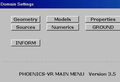
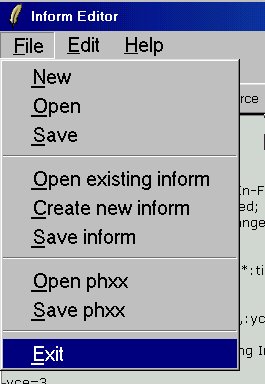
One such button is shown here, for the top panel.

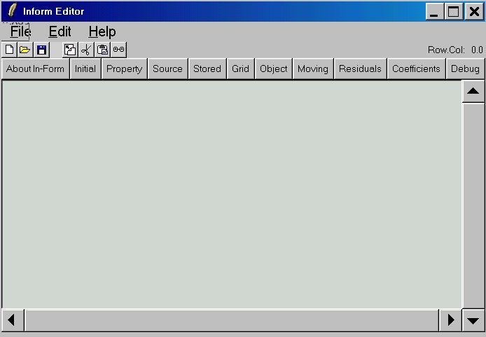
When that button is pressed, the Inform Editor appears.

Similar buttons appear on lower-level panels of the VR-Editor user-interface.

(c) Example; library case 360

There now follow several screen-capture images which show stages in the editing of the moving-body trajectory.

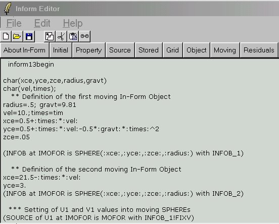
The existing Group 13 statements are viewed here

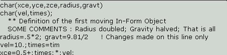
They are then changed by way of Notepad-like editing actions to this.

When they are what the user wants, they are saved.

This action places them in the phxx file which the VR Editor uses to store items which must be written to the final Q1, the relevant part of which is seen here:


  Echo InForm settings for Group 13
  inform13begin
char(xce,yce,zce,radius,gravt)
char(vel,times);
   ** Definition of the first moving In-Form Object
   SOME COMMENTS : Radius doubled; Gravity halved; That is all
radius=.5*2; gravt=9.81/2     ! Changes made on this line only
vel=10.;times=tim
xce=0.5+:times:*:vel:

(d) The future of the Inform Editor

The VR and In-Form Editors work satisfactorily together.
However, it will take some time for the maturity of the former to be emulated by the latter, and for the In-Form Editor's greater flexibility to be utilised by VR.
The In-Form Editor needs at least two additions before it can be considered mature, namely:
1. It must enable suitable formulae to be selected from lists in drop-down menus; and
2. it must subject what is typed in to immediate validity checks, and then reject, with advice, syntactical errors.
What it can offer to the VR-Editor is the ability to handle:
- PIL declarations,
- IF statements and
- DO loops; and indeed
- all the excellent PIL features which the current VR-Editor disregards.
Now that the PHOENICS Commander, which also employs the Tcl/Tk package, has been adopted as the main introduction to and manager of PHOENICS, these additions to the In-Form Editor will swiftly be made.

Back to main contents

12. Adjustment of terms in differential equations

The GROUP 12 feature of PHOENICS allows the diffusion, convection and source terms in the differential equations solved by PHOENICS to be altered from their standard formulations.

In-Form can effect more extensive modifications of these terms; morever it does so without the use of special patch names.

12.1 How to modify diffusion and convection terms

The (moddif ...) or (modcon ...) keywords of In-Form are placed at the beginning of an In-Form statement, the purpose of which is to introduce new value of diffusion or convection terms into the balance equations of solved-for variables, i.e. those which have featured in a preceding SOLVE(), or SOLUTN(name,y,y,....) statement.

The recalculation will be executed only at internal cell faces of the domain area; for updating at domain boundaries, the moddif and modcon statements can not be used.

The complete format of the In-Form moddif and modcon statements is:

(MODDIF OF varname AT patchname IS formula WITH options)
and
(MODCON OF varname AT patchname IS formula WITH options)
where:
- 'varname' is the name of the solved-for-variable;
- 'patchname' is the name of a patch defined by a preceding (in the q1 file) PATCH statement, which defines the limits, in terms of ixf, ixl, iyf, iyl, izf, izl, itf and itl, within which the calculations are executed.
  The type of patch has no significance;
- 'options' specify names of cell faces where the modification is executed.
  Possible names are EAST, NORTH and HIGH.
  If the options are absent, the calculations are executed at all cell faces.
- formula is the mathematical expression of new diffusion or convection terms.

12.2 How to modify built-in source terms

Similarly to the previous section the (modsor ...) keyword of In-Form is placed at the beginning of an In-Form statement, the purpose of which is to make adjusment of value of built-in source terms into the finite-volume equations of solved-for variables.

The complete format of the In-Form (modsor statements is:

(MODSOR OF varname AT patchname IS formula)
where:
- 'varname' is the solved-for variable name;
- 'patchname' is the name of a patch defined by a preceding (in the q1 file) PATCH statement. The type of patch statement has no significance;
- 'formula' is the mathematical expression of new source term.

In modsorq1 case In-Form is used to simulate flow near the thin pipe grid which is placed horizontally at north faces of cells for each iy=iysh. The diameter of pipes is very small and equal diam=0.01 m. Thus the pipe grid is a subgrid object. It is supposed that the pressure drop at pipe grid can be calculated by formulas


  dP = f*2*rho*vel^2, [N/m^2]
  f=0.33*Re^(-1/5)    and
  Re=abs(vel)*diam/enul

The resistance at the pipe grid is simulated by updating the built-in source term of equation for v1 variable at iy=iysh cells by means following two lines


 PATCH(MSOR1,CELL,1,NX,IYSH,IYSH,1,NZ,1,1)
 (MODSOR of V1 at MSOR1 is ANORTH*.33*REYN^(-0.2)*2*RHO1*VLSQ)

End of main text of In-Form Documentation

Back to main contents

9. Print-out-related capabilities

Contents of Section 9

9.1 The LONGNAME keyword

Syntax

An earlier 'longname' feature

9.2 The PRINT keyword

Syntax

First example

Line-printer plots in RESULT

Printing arrays

9.3 Coefficients, residuals, corrections and exchange coefficients (gammas)

Coefficients

Residuals

Corrections

Warning

Exchange coefficients (gammas)

Manipulating the coefficients, etc

9.4 Eliciting debug

9.5 Tabular Output

10. Replacing READQ1

(a) REALREAD, INTREAD and LOGREAD

(b) Discussion

11. In- Form and the VR-Editor

(a) Historical background

(b) Editing In-Form statements via the menu

(c) Example; library case 360

(d) The future of the Inform Editor

12. Adjustment of terms in differential equations

12.1 How to modify diffusion and convection terms

12.2 How to modify built-in source terms

End of main text of In-Form Documentation