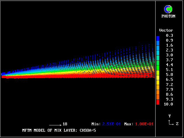
 Here are the velocity vectors
Such layers have been much studied, both experimentally (eg by Reichardt, 1942) and theoretically (eg by Tollmien, 1926). It is known that the profile approximately fits the formula:
W' = [ 5 * Y' ** 2 - 2 * Y' ** 5 ] / 3
MNSQ is defined as the local root-mean-square velocity fluctuation.
Its cross-stream width increased from nearly zero to 0.725 m at a distance of 3.12 m from the start.
The flow-direction velocity of the entering stream, designated as fluid 1, was 10 m/s; the reservoir fluid, designated as fluid 40, had a flow-direction velocity of zero.
These fluids entered the wedge-shaped computational domain, through its two inclined boundary surface, at the rates necessary to ensure conservation of momentum, total mass, and the satisfaction of the transport equations of all 40 fluids. They were outcomes of the calculation rather than bondary conditions.
The calculations were performed by the PHOENICS code, working in parabolic mode. The calculation took 642 seconds on a Pentium 200 PC.
So one does not have to wait long for results, some of which now follow. [The date may be noteworthy; it is that of the first- ever hydrodynamic-flow calculation based on MFM]
First, some velocity-vector concentration-contour plots will be shown. These will be followed by some computed PDFs.
The above-mentioned results are those of the 1996 calculation. Nowadays such calculations are routine, there being a mixing-layer example in the latest PHOENICS Input-File library.
The cross-stream profiles shown below come from the library case.
The velocity vectors are as expected.
The grid is an expanding one, with 40 intervals across and 100 along the layer.
 Here are the velocity vectors
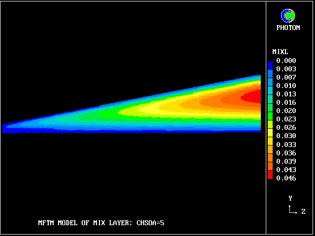 This is the distribution of the computed length scale
and this is
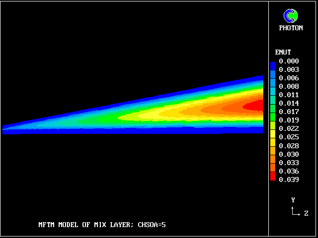 the computed effective-viscosity distribution
Agreement with experiment is good.
The following picture shows contours of the average concentration (for all 40 fluids) of material emanating from the upper stream.
It is just as a conventional turbulence model (eg mixing-length or k-epsilon) would reveal; but no transport equations for statistical quantities are being solved.
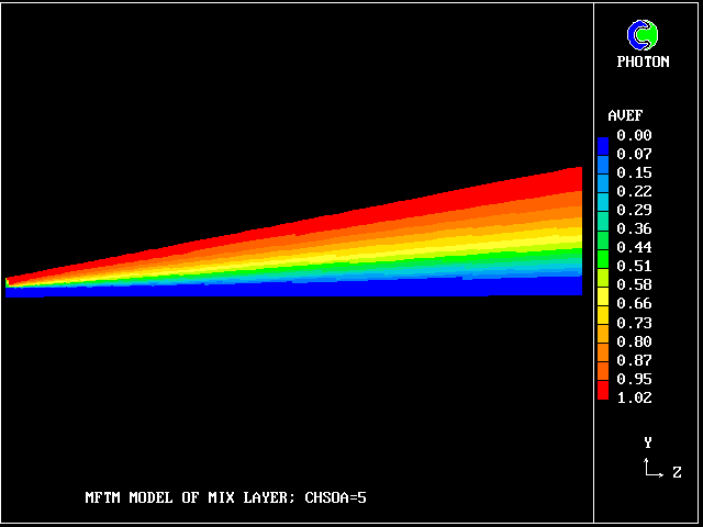 average concentration of material
from the upper stream
But how much upper-stream fluid (fluid 40) remains in its pure state? Only this.
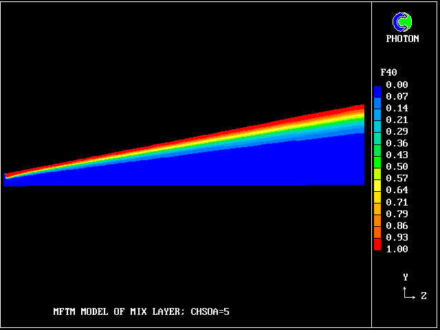 concentration of upper-stream fluid (fluid 40)
Where has the rest gone?
What about pure lower-stream fluid?
It also occupies very little space.
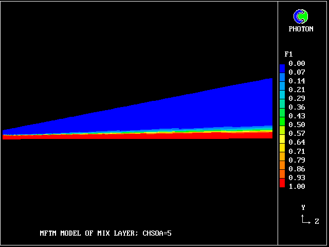 concentration of lower-stream fluid
So what lies in between? 38 other fluids, variously intermingled.
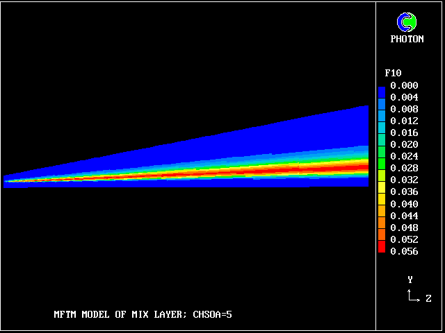 The contours for fluid 10
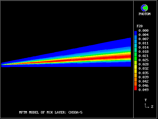 The contours for fluid 20
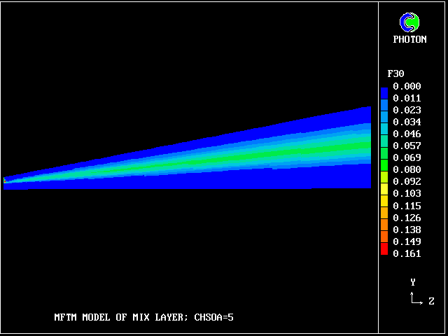 The contours for fluid 30
The results can be processed and displayed in many different ways.
Particularly relevant to the theme of the present paper are the discretized probability-density functions (PDFs), which may also be called:
Fluid-Population Distributions (ie FPDs) .
The PDFs are on the left in the next pictures.
The displays on the right are reminders of how the population of fluids might be distributed in a single computational cell, namely at random.
All the PDFs to be shown relate to a downstream section of the mixing layer, where the profiles are fully developed.
The first relates to a location near the lower (higher-velocity) edge of the layer.
The population consists almost entirely of higher-velocity fluid
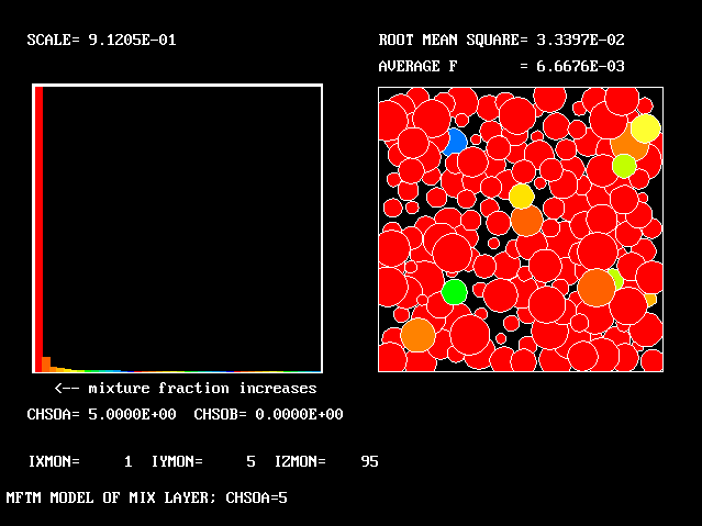 higher-velocity edge
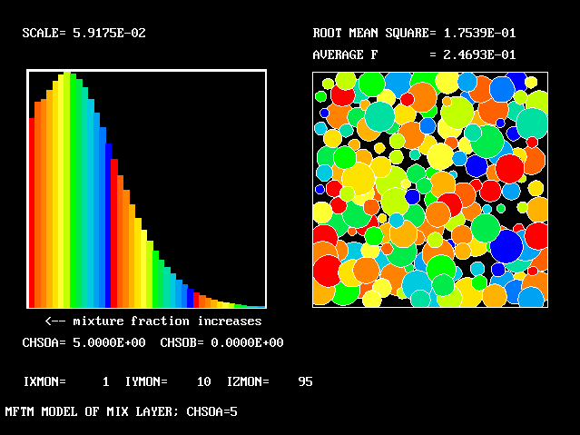 At 1/6 of the width from the higher-velocity edge
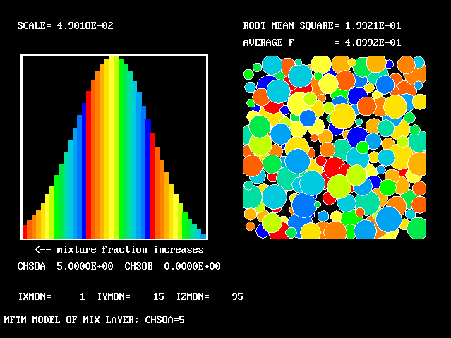 At 2/6 of the width from the higher-velocity edge
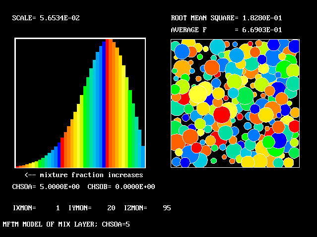 At 3/6 of the width from the higher-velocity edge
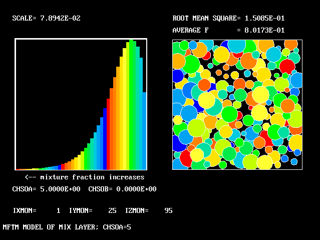 At 4/6 of the width from the higher-velocity edge
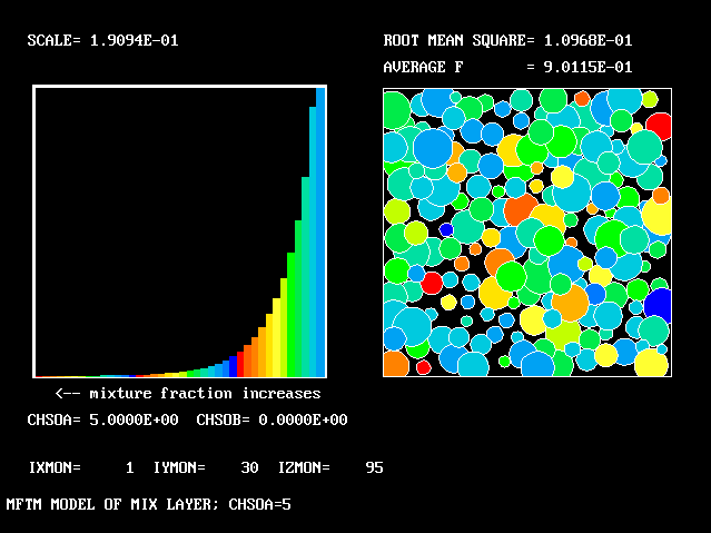 At 5/6 of the width from the higher-velocity edge
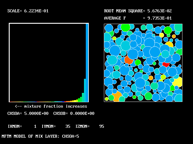 At a location very near the lower-velocity edge
All that has been used so far is the root-mean-square velocity fluctuation, as an input to the formulae for:-
As expected, a self-similar distribution is found.
The value along the "spine" of the layer is approxinately 20 % which is in order-of-magnitude agreement with experimental data.
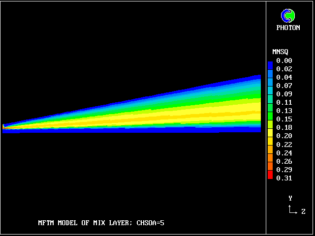 contour plot of MNSQ
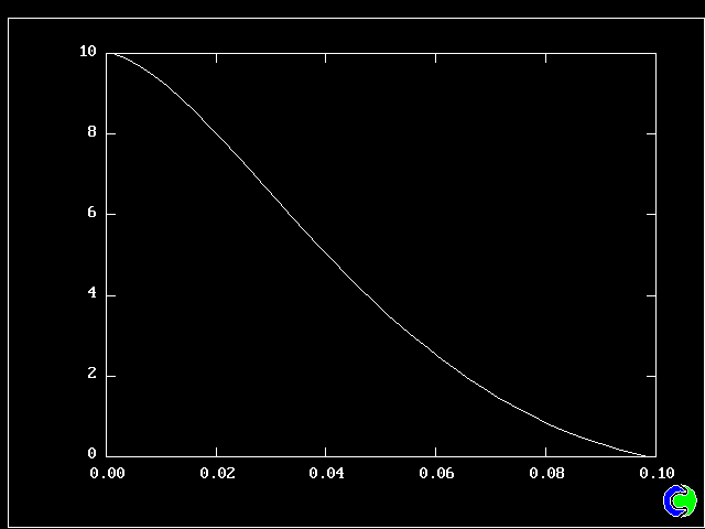 Fig 8.2.1 The population-mean longitudinal velocity
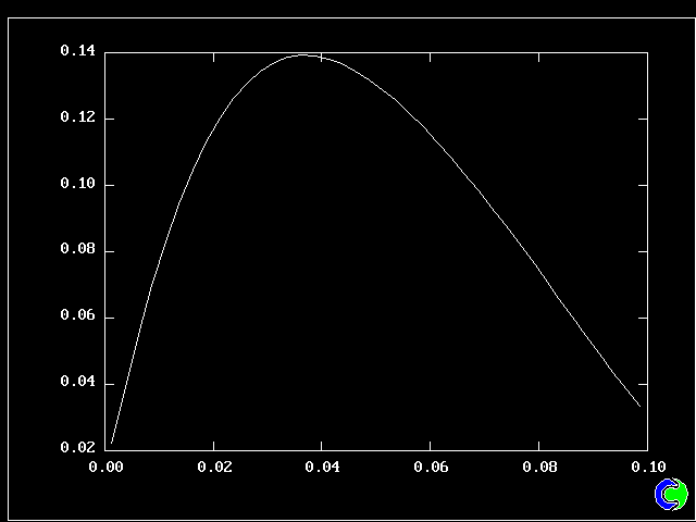 Fig 8.2.2 The root-mean-square velocity fluctuation
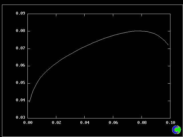 Fig 8.2.3 The profile of the length scale
 Fig 8.2.4 The profile of effective viscosity
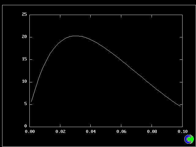 Fig 8.2.5 The profile of the coupling-splitting rate
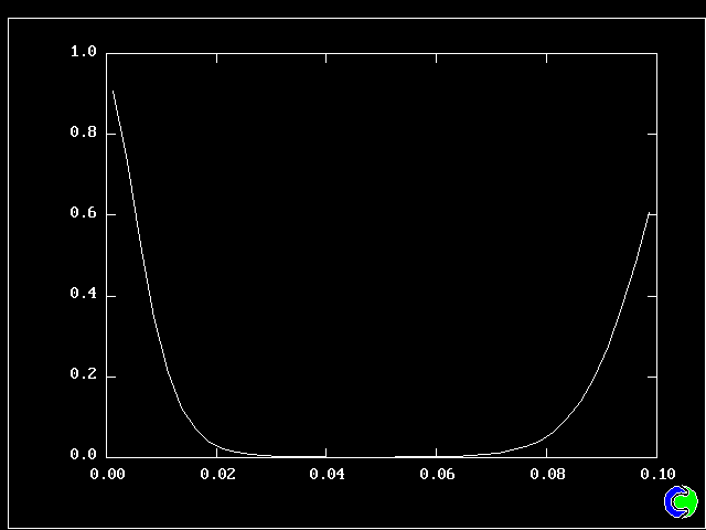 Fig 8.2.6 Concentration profiles of entering and reservoir fluids
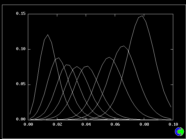 Fig 8.2.7 Concentration profiles of some intermediate fluids
The width is here defined as the distance across the layer between the points where the mean velocity is 0.1 and 0.9 times the maximum velocity. With this definition. the rate of-spread ratio is found to be: 0.153 .
Other numerical results of interest are, for the fully-developed region, the following dimensionles numbers:
8.3 Comparison with experimental data
(a) Rate of spread, etc
An experimental investigations by Reichardt (1942) has shown that:-
Passive-scalar profiles are not exactly the same as longitudinal- velocity profiles in plane mixing layers, but have the less-curved shape which corresponds to an effective Prandtl number of less than 1.0.
Nevertheless, it is gratifying to note that the shapes of the PDFs reported by Batt are in qualitative accordance with those presented above, varying from near-symmetry in the centre of the layer to marked "lopsidedness" near the edges of the layer.
It may also be of interest to note that Fueyo et al (1995) reported a numerical study of the mixing layer by means of a Monte-Carlo- based method. Their reported PDFs were similar to those of the present paper; but the computer time, with 600 computational cells compared with the present 4000, was 45 minutes on a Convex C220 .
In particular, the multi-fluid model predicts the overall flow characteristics as well as a conventional model; and, because it computes the PDFs, as a conventional model cannot, it provides much more detailed insight into (what may be) the physics of the flow.
Nevertheless, no investigation has yet been made as to whether the constants which were found appropriate for the mixing layer will serve also for other flow situations.
Further, it needs to be established whether the discretization was adequately fine, in respect of the finenesses of the both the geometric and population grids. The PHOENICS library case facilitates this.