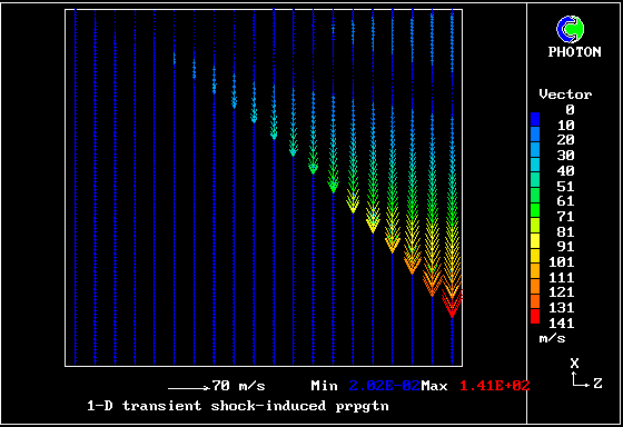
 Velocity vectors of the cooler gas
This belief led to searches for labour-saving schemes, based upon
the presumptions that:
either
the PDF has a known, simple shape;
or
certain statistical properties of the PDF will suffice.
Both of these will be discussed in this section.
(a) The eddy-break-up model (EBU), (Spalding, 1971)
The eddy-break-up model for turbulent combustion represents the population distribution by two spikes, as shown:
              |
       mass   |   ^unburned
       fractions  |
       of the |   |
       two    |   |                ^burned
       gases  |   |                |
              |   |                |
              |   |                |
              |   |                |
              |___|________________|_____
                  0  reactedness-> 1
At any location, the gas
mixture is supposed to
comprise fully-burned and
fully-unburned gases.Their proportions vary with location in accordance with laws of convection, diffusion and source/sink interactions.
The latter represent the transformation of unburned to burned at a volumetric rate proportional to the local mean-flow shear rate.
In some variants, a chemical-kinetic rate-limitation was introduced.
The eddy-dissipation concept model for turbulent combustion also presumes a two-spike population distribution, represented as shown:
              |
       mass   |         ^mean mixture
       fractions        |
       of the |         |
       two    |         |
       gases  |         |
              |         |
              |         |    ^fine
              |         |    |structures
              |___|_____|____|_____|__
                  0  reactedness-> 1
At any location, the gas mixture is supposed to comprise mean mixture and "fine structures",
Their proportions vary with location in accordance with laws of convection, diffusion and source/sink interactions.
The latter involve mass transfer between the two gases at a volumetric rate proportional to the local mean-flow shear rate.
Chemical kinetics controls the rate of fine-structure reaction and so the mean-mixture reactedness.
The two-fluid model of turbulent combustion presumes a two-spike population distribution, represented as shown:
              |
       mass   |         ^slower fluid
       fractions        |
       of the |         |
       two    |         |
       gases  |         |
              |         |
              |         |    ^faster fluid
              |         |    |
              |___|_____|____|_____|__
                  0  reactedness-> 1
At any location, the gas mixture is supposed to comprise faster- and slower- moving gases.
Their speeds & proportions vary with location in accordance with laws of convection, diffusion and source/sink interactions.
The latter involve mass transfer between the two gases at a volumetric rate proportional to the local relative velocity.
Chemical kinetics controls the rate of chemical reaction within each gas, and so their individual reactednesses.
A shock wave passes down a vertical pipe containing a combustible gas which is burning slowly.
The wave accelerates the hot-gas fragments more than the cold ones, causing relative motion.
The relative motion causes increased entrainment and mixing, which leads to increases in the burning rate.
The increased rate increases the strength of the pressure wave.
The result is that the deflagration turns into a detonation.
The graphical plots show the development, the horizontal dimension being time.
The calculation was first performed in 1983. Its specification may be found in the PHOENICS Input-file library (case 893).
 Velocity vectors of the cooler gas
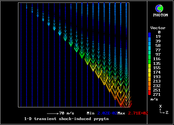 Velocity vectors of the hotter gas, which has been more greatly accelerated
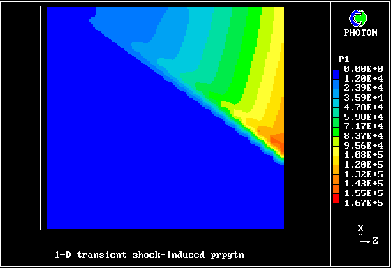 The contours of pressure
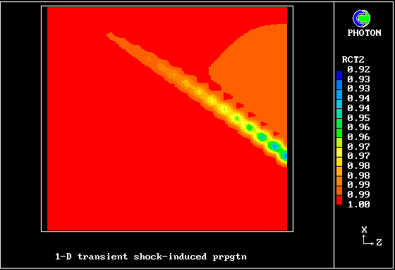 The reactedness of the hotter gas
A steady stream of turbulent pre-mixed combustible gas flows into a parallel-walled duct. A flame, anchored by a centrally-placed flame- holder, spreads to the walls.
The parabolic-flow option of PHOENICS has been used for solving the four momentum equations, two energy equations and two mass- conservation equations.
The empirical constants employed concerned:-
The simulation featured in the Imperial College research of Jeremy Wu, 1987. It is now PHOENICS Input Library Case no W977. Agreement with experimental data, eg Williams, Hottel and Scurlock, is good.
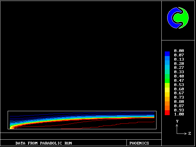 Contours of reactedness of the faster fluid.
The flow is from left to right.
Only the upper half of the duct is shown.
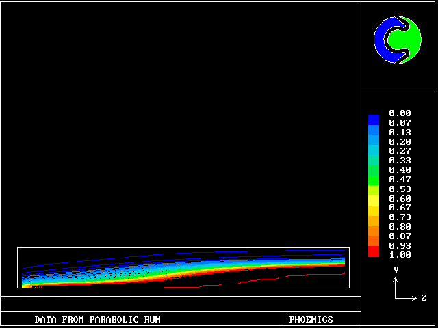 Contours of reactedness of the slower fluid.
These contours differ from the previous ones, in that the cooler (slower-moving) fluid is the less reacted.
The two-fluid turbulence model is of use for other phenomena than combustion, and especially for those in which density differences interact with body forces.
Many examples arise in the atmosphere, lakes, rivers and oceans.
The two-fluid model, for example, can satisfactorily simulate the mixing-followed-by-unmixing behaviour when a salt-water layer, lying below fresh water, is heated for a short time.
            _________      _________      _________
           |         |    | * ** *  |    |         |
           |  fresh  |    |* *  * **|    |         |
           |         |    | * ** *  |    |         |
           |*********|    |* *  * **|    |*********|
           |* salty *|    | * ** *  |    |*********|
           |*********|    |* *  * **|    |*********|
            ---------      ---------      ---------
              start         later           later
                                            still
Mixing appears to take place soon after heating equalises the densities. But it is macro- not micro-mixing; so "unmixing" follows.
Experiments by Spalding and Stafford at Imperial College during 1979, in which the heating was effected by passing an electric current through the fluids, brought the mixing/unmixing phenomenon to light.
It was consideration of these experiments which prompted the development of the two-fluid model of turbulence, which has here been used to simulate it.
In this and the following pictures, which show contours computed by way of the two-fluid turbulence model:
The first picture shows
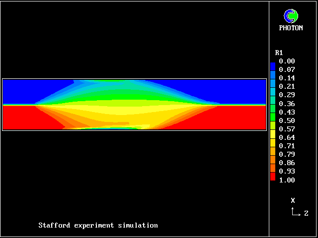 the volume fraction of lower (saline) fluid.
Note the initial delay; then mixing; then unmixing.
This picture shows how
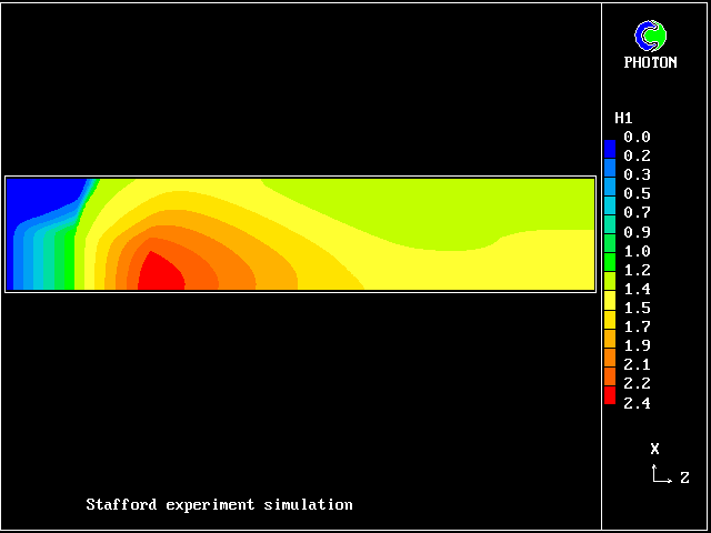 the temperature of the saline fluid
first rises; it falls later, as heat is transferred to the
fresh-water fluid.
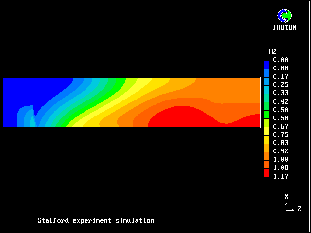 This picture shows how the fresh-water temperature rises,
gaining its heat from the saline fluid.
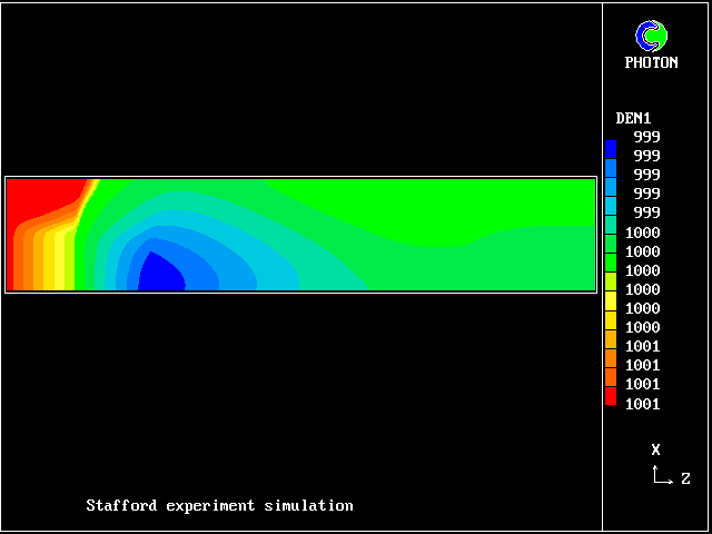 Here is shown the density of the saline fluid.
It first diminishes, because of the temperature rise, eventually
becoming lighter than the fresh water.
As it cools, it becomes heavier again.
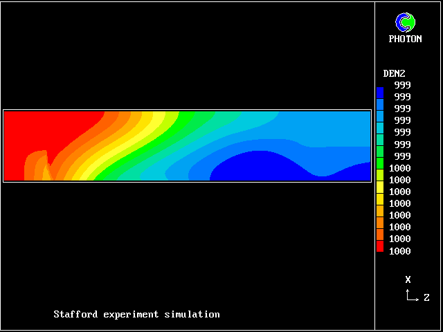 Here is shown the density of the fresh-water fluid.
This also diminishes, as heat is transferred from the saline
solution; but it also increases later because some salt
diffuses into it.
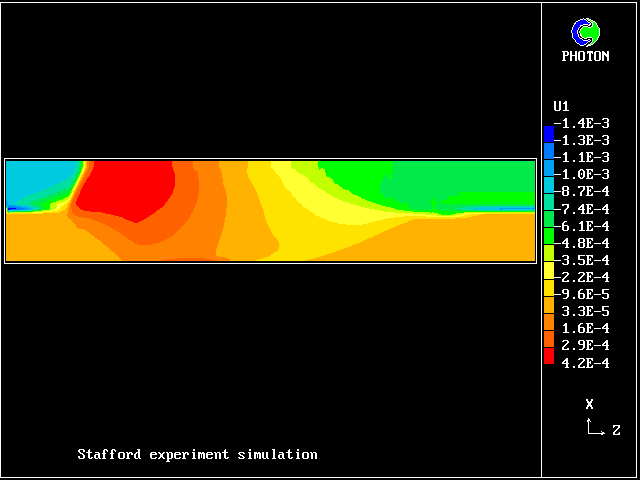 This picture shows how the vertical velocity of the saline
fluid becomes positive, once its density falls below that of
the fresh water.
Here are the corresponding
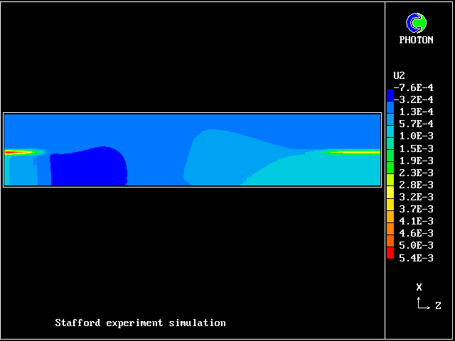 vertical-velocity contours of the fresh water
Later, cooling causes it to become negative again. Reminder: the horizontal dimension is time, increasing to the right.
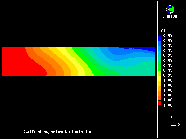 The salt content of the lower fluid does diminish somewhat
in the course of time.
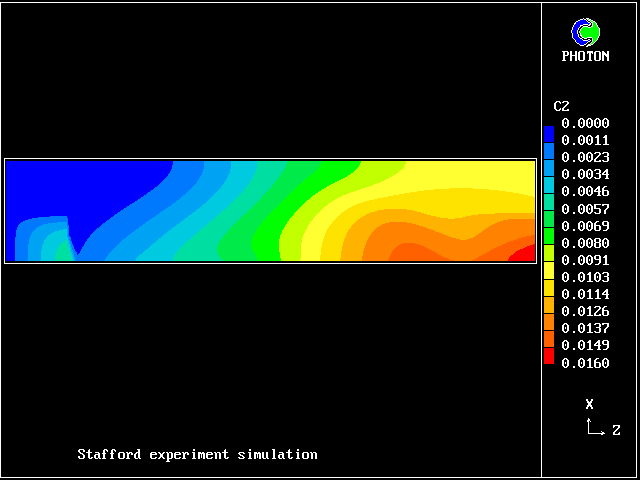 The salt content of the upper fluid correspondingly
increases.
Click here for more about the two-fluid model
The simulation agrees qualitatively with the observations; but the "two-spike" representation of the fluid population is too crude for anything better.
Conventional turbulence models, for example k-epsilon, RNG, Reynolds-stress, etc cannot provide even qualitative agreement; for they lack the multi-fluids-in-relative-motion concept.
Phenomena of this kind are significant in many environmental phenomena, especially in the oceans.
The above-mentioned flames have concerned pre-mixed flames; but PDF shapes are often presumed for pre-mixed ones as well, the simplest presumption being the symmetrical-two-spike one.
       mass   |
       fraction
       of the |_0.5
       two    |         ^    ^
       gases  |         |    |
              |         |    |
              |         |    |
              |         |    |
              |___|_____|____|_______|_____
                  0 fuel fraction &  1
At any location, the gas
mixture is supposed to
comprise gases equally more
and less rich than the mean,
their deviations from the
mean being computed by way
of a transport equation for
the RMS fluctuations. Then the compositions of each gas are computed from the "mixed-is- burned" presumption.
Later authors have made more complex presumptions about the shape of the PDF, for example "clipped-Gaussian" or "beta-function".
These increase the amount of computation which is needed, sometimes very greatly; but it has not been demonstrated that the extra work is rewarded by improved realism of predictions.
As will be shown below, PDFs can vary greatly in shape from one part of a flame to another. Therefore, while two-spike models are useful because they promote physical insight with small computational cost, it can be argued that the more complex models increase obscurity rather than realism.
In any case, for non-pre-mixed turbulent flames, the PDF should be two- rather than one-dimensional, as will be explained below.
Currently popular turbulence models rely upon the presumption that all that needs to be known about a PDF is a few of its statistical properties.
AN Kolmogorov (1942) first proposed this; and he also postulated that two such properties, namely the energy and the frequency of the turbulence, obey differential equations of "transport" type, involving:
time-dependence, convection, diffusion, creation & destruction.
Later authors have employed different variables, eg:
(as just mentioned)
For fuller information about conventional turbulence modelling, see
the article on turbulence modelling in the PHOENICS Encyclopaedia.
Nevertheless, methods of this (ie Kolmogorov-style) kind perform rather poorly for hydrodynamic phenomena when body forces (gravity, or centrifugal) are significant (as in Stafford's experiment); for they lack the "unmixing-because-of-body-forces" element.
Moreover they do not provide for calculation of the shapes of the PDFs, which are essential if chemical reaction is to be simulated.
Fortunately, despite popular belief, the Kolmogorov approach is not the only one which is available, as will be explained below.
Click here to continue browsing through the lecture or here to return to the start.